
Abstract
1. Objective
The aim of this study was to identify, delimit and estimate the thickness of the oceanic and continental crusts in the Farallon Basin in order to understand the geological processes that occur during the continental lithosphere’s rupture and the deformation of passive margins. In order to achieve this objective, the following specific goals were defined:
- Process, interpret and identify high resolution 2D multichannel seismic reflection data from the seismic profiles;
- Create gravimetric models from the main measurements interpreted in the seismic profiles;
- Estimate the depth of the Basement supported by gravimetric data;
- Estimate the thickness of the crust in the area.
2. Seismic reflexion method
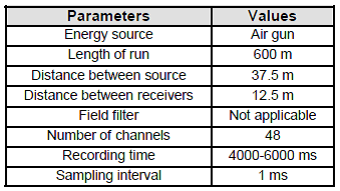
A marine linear array (Figure 1) was used for data acquisition. For this purpose, a 150 cubic inch (0.245m3) per shot airgun was used as the energy source (see Table 1).

3. Seismic Data Processing
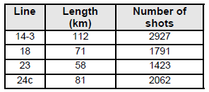
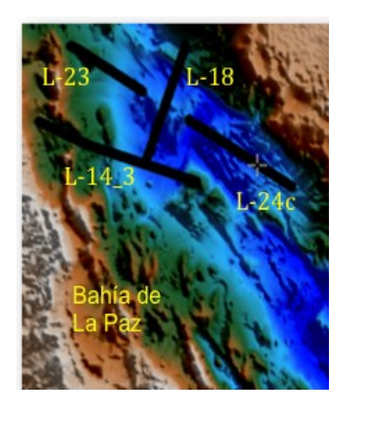
Data from four seismic lines from the Ulloa-6 campaign (Table 2 and Figure 2) were processed using the ProMAX software of the Landmark software platform. The processing sequence shown in Figure 3 used a typical reflexion seismic processing sequence described by Yilmaz (1987) and Sheriff and Geldart (1995).

Once the seismic process sequence was finished the interpretation of the seismic line was performed (Figure 4).

After the four seismic profiles were processed and interpreted, a Basement’s type distribution map was generated using the seismic data collected in the area of study (Figure 5).

4. Potential Field Methods (Gravimetric Method)
The gravimetric method of geophysical exploration is based on the measurement of small variations of the earth’s gravitational field on its surface and their interpretation in relation to possible mass distribution in the subsurface (Nettleton, 1976). The gravimetric observations can be used to interpret changes or differences of mass below different regions of the earth (Lillie, 1999).
A first step is to isolate the gravity field fraction originated by these mass differences. This is the reason calculating the Free-Air gravimetric anomaly (Figure 6 – left). Second, in order to remove the gravimetric effect generated by the sea and the land in the area of study, the gravimetric anomaly of Bouguer was calculated (Figure 6 – right).
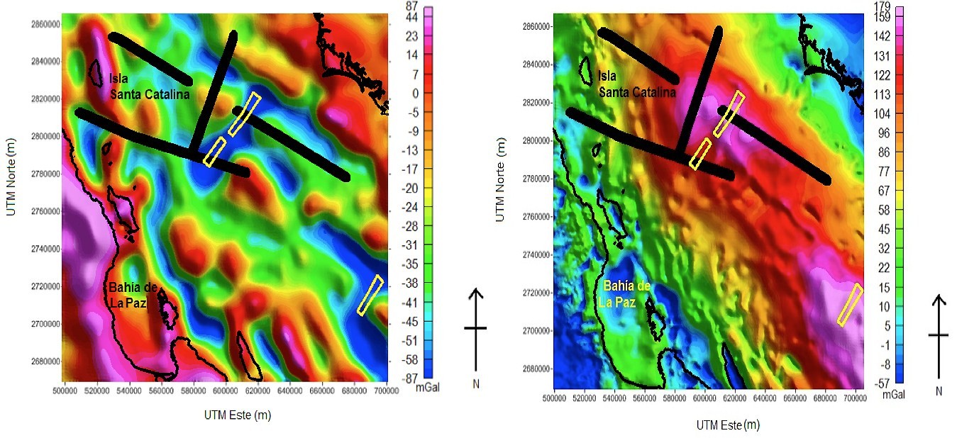
Lines show the seismic profile locations.
5. 2D Modelling
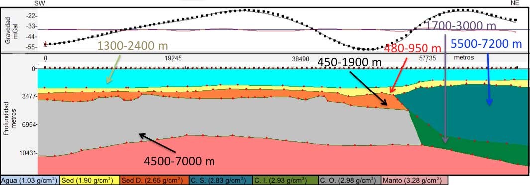
The Free-Air gravimetric data was used to generate subsurface models. To compile these models, the depths of the main interpreted reflectors of the seismic sections, the general characteristics inferred from the qualitative interpretation of the gravimetric anomalies’ maps as well as the gravimetric data itself were used. A trial and error adjustment was used in the bi-dimensional case obtaining models of the four seismic profiles (Profile 18 is shown in Figure 7).
6. 3D Inversion
To perform the 3D gravimetric inversion of the data the GMLayers software (Gallardo et al., 2005), as amended in October 2010, was used. To guide the inversion process using the GMLayers software, it is necessary to set up a number of parameters grouped as:
- initial model;
- precision of the initial model and the geophysical data;
- acceptable smoothness level of each surface; and
- the feasibility limits of the thickness and depth of each layer of the model (as shown in Figure 8).
The appropriate setting of theses parameters is key to obtaining an optimum model that not only justifies the data, but retains its geological meaning.
In Figure 8, the s2 surface (black line) corresponds to the bathymetric relief which is always located above the s4 depth ranges. In this case, the upper surface is fixed at 0 km (sea level) and the effect of the sea level is suppressed, hence the minimum and maximum thickness of the overlying layer match the minimum and maximum depths in the area. In both cases it is possible to observe the seismic profile’s restrictions given by depth.
After the program was run and the results checked, the anomaly obtained in the field was compared against the one calculated by the program. It was observed that their differences were minimal (Figure 9) which can be explained by the limitations of the seismic pro- files.


7. Layer Structures
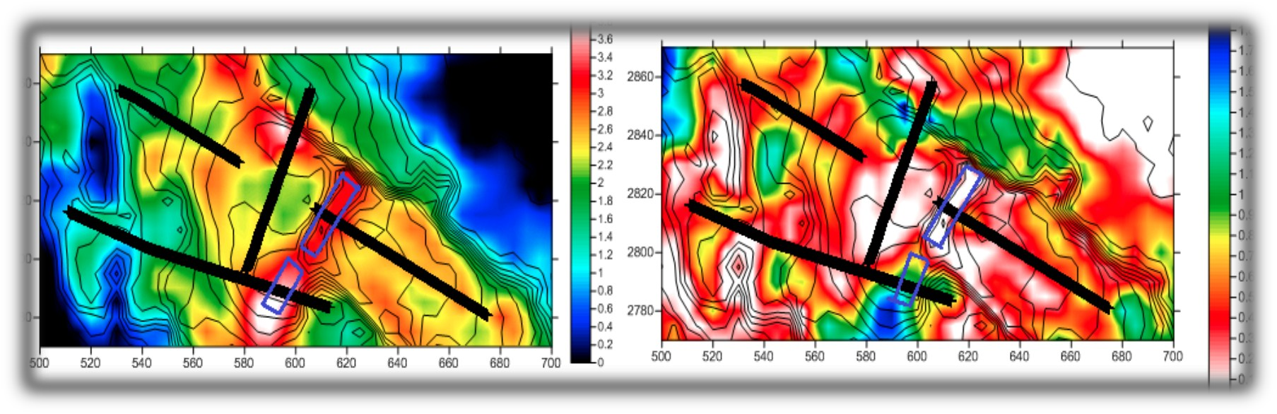
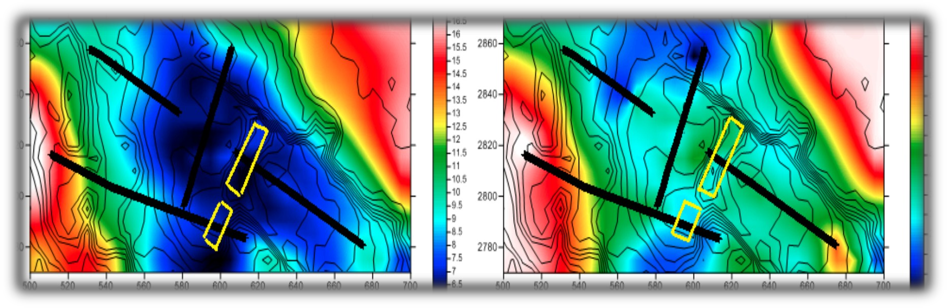
Figures 10 to 13 show the thickness of the various layer structures (km).
a. Sediments

b. Continental crust

c. Oceanic crust
8. Conclusions
The integration of seismic data, potential fields and 3D gravimetric inversion identified the type and structure of the crust in the study area. The different thicknesses and distribution of each identified layer were compatible with the tectonic scenario as follows:
- In the uppermost part it was observed that the active axis of the Farallon Basin, at a depth of 3.2 km, does not present sediments; whereas, the abandoned axis, at a depth of 3.8 km, it is buried by a sedimentary package with a total thick- ness of 2.9 km.
- Evidence suggests that the sedimentary material which overlays the recently created oceanic crust is affected by magmatic intrusions. This was not detected in the sediments deposited on the continental crust.
- On the western zone, it was observed that a continental crust with a thickness of 15 to 17 kms thins towards the centre of the basin. At that point it is almost entirely replaced by a thin oceanic crust of recent creation which has a thickness of 2.7 to 6 km.
- Finally, the rise of the mantle layer in the rift areas is clearly observed, reaching 5.8 km on the active axis and 7.3 km on the abandoned axis. A deepening was observed towards the continental zone which corresponds to the margins of the Gulf of California.
9. References
Gallardo, L.A., Perez, M.A., Gomez, E. (2005). Refinement of three-dimensional multilayer models of basins and crustal environments by inversion of gravity and magnetic data. Tectonophysics, 397, 37-54, doi:10.1016/ j.tecto.2004.10.010.
Lillie, R. J. (1999). Whole earth geophysics: an introductory textbook for geologists and geophysicists. Upper Saddle River, Prentice-Hall, New York.
Nettleton, L. (1976). Gravity and Magnetics in Oil Prospecting. McGraw-Hill, New York.
Sheriff, R.E., Geldart, L.P. (1995). Exploration Seismology. Cambridge University Press. 2nd Edition. New York, NY.
Yilmaz, O. (1987). Seismic data processing: Society of Exploration Geophysicists. Tulsa, OK.
10. Biography
Lieutenant Marco Bartens graduated from the Naval School of Peru in 2006 and completed his IHO Category B certification in 2008 whilst working in the various divisions of the Hydrography Department. In 2011, he was promoted to Second Lieutenant and commenced his specialization studies at the Cientific Investigation Center for Superior Studies of Ensenada (CICESE), Mexico. He graduated in 2013 with a Master of Science, specialization in Applied Geophysics. In 2015, he was promoted to First Lieutenant and is now working as the Deputy Chief of the Oceanography Department of the Peruvian Directorate of Hydrography and Navigation.