
Abstract
1. Introduction
This investigation was a practical application of the well-known inverse problem of geodesy – using the great long line geodesic formulae to determine the station’s position and ensure that the accuracy requirements for the OMEGA signal could be met. OMEGA is a Very Low Frequency (VLF) hyperbolic system with world coverage, where for a Line of Position (LOP) is defined as being the line along which the difference of distances of each point to the pair of stations used in the system is constant Using the known wave length of the system, the difference of distances can be converted into a correction reading using appropriate formulas.
The OMEGA wave length was 29478.087 meters and a constant of 900 was added for obtaining each reading. The same parameters were used in reverse to obtain the difference of distances from a reading. In the proposed observation design, each series of observations consisted of a set of three pairs of readings recorded hourly for the stations of Lagos (Mainland), Porto Santo (Madeira Islands) and Horta (Azores Islands).
The distances between OMEGA stations are several thousands of kilometers. To determine the positional errors, distance calculations between the stations used long line geodesic solutions with the inverse problem of geodesy. This could be achieved once the positions of the OMEGA stations were known along with the differential positions of those stations. The goal was to obtain calculated distances to compare with those obtained by the readings. To determine each observed point, the method of “variation of coordinates” was used with compensation by mean squares calculation. For each month, a statistical treatment was undertaken. The known positions of the OMEGA stations were then compared with the station’s observed coordinates.
The time series of the readings were taken and converted into difference of distances between the differential stations and those of the stations of the OMEGA system. The calculated distances were computed with the long line geodesics using the rigorous method of Wallis Integrals. These positions were then compared with the positions given by the readings in the stations and deviations were computed.
Part of the analysis resulted in a number of statistical parameters being computed and displayed. This included a Scatter Plot with the 95% dispersion ellipse and the Relative Frequency Diagram for the several frequency ranges of each group of distances between the calculated and observed points in the stations. This analysis took into consideration the various physical parameters that affect accuracy of the overall OMEGA system. With this study, it was then possible to confidently determine the appropriate correction factors to be broadcast.
2. Calculation Methods
The fundamental method consists of calculating the differential of the difference of distances, considering possible environmental errors associated with VLF continuous wave electromagnetic signals (e.g. propagation, noise, instrumentation, signal correlation, etc.) In one reading for a distance, we have the observation equation:
dD + Dc – Do = r (1)
Where:
dD – differential of the distance
Dc – calculated distance (real distance to the stations of the system)
Do – observed distance from a reading
r – residual
If we measure the difference of distances of the stations in the system, a and b to the differential station f, we have:
dDa – dDb + (Dca – Dcb) – (Doa – Dob) = ra – rb = rf (2)
This is the basic observation equation.
The difference of the observed distances can be obtained from the reading Lab as:
Doa – Dob = (Lab – 900) * 29478.087
The difference of the calculated distances is obtained from the long line geodesic calculations between each of the stations in the system and the reading station, whose coordinates are all known. The coordinates were referenced to the WGS72 ellipsoid.
In conjunction with the long line geodesics, precise solutions as those of the Wallis Integrals (Pasquay, 1972) and (Rapp, 1981) are adopted. These are defined in the Jacobi´s sphere or parametric sphere, which implies a representation of respective angles (azimuths) rather than distances, latitudes or longitudes. However, the geodesics match point to point. The spherical latitudes or reduced latitudes can be obtained through the formula:

(3)
Where:
L – geographical latitude (in the ellipsoid)
L’ – spherical or reduced latitude (in the sphere)
a – semi-major axis of the ellipsoid
b – semi-minor axis of the ellipsoid
The longitudes calculation is difficult to resolve. The computation starts from the difference of longitudes and is corrected by an iterative method. This process determines the correction (p), variation of the difference of longitudes between the two extremities of the geodesic, when you pass from the ellipsoid to the sphere and using the difference of the elongations wa and wb as the value for the first approximation. This is then corrected by the iterative method.
We have then:
DG’ = DG + p or
p = DG’ – DG (4)
Where:
- DG’ – difference of longitudes in the sphere
- DG – difference of longitudes in the ellipsoid
- p – correction obtained by the iterative method
Clairaut’s Equation establishes the constant relationship:
cos L'(a)*sin A(a) = cos L'(b)*sin A(b) (5)
Where:
A(n) – azimuth of the geodesic in the point n (either a or b)
As mentioned later in this paper, the azimuths are now the same in the ellipsoid and in the sphere.
So:
A'(n) = A(n).
The element of the meridian in the ellipsoid and in the sphere is:
R * dL = ds * cos A and dL’ = dw * cos A
The element of the parallel is also:
r * dG = ds * sin A and cos L’ * dG’ = dw * sin A
Where:
- r = a * cos L’ (radius of the parallel in the reduced latitude L’)
- dw – element of the arc of the great circle in the sphere
- ds – element of the geodesic
- R – curvature radius of the meridian
- dG – element of longitude in the ellipsoid
- dG’ – element of longitude in the sphere
Considering the square of the 2nd eccentricity:
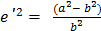
And also:
V2 = 1 + e’2 * cos2 L’
We have:

differencing the formula (3)
As we have also along the meridian:

And also:

We have:

(6)
And:
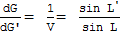
or
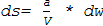
(7)
To obtain the required accuracy in the distance, we have to integrate the element of the arc of the great circle dw in the sphere through formula (7). Integrating this formula from point a to b along the geodesic and using the Wallis Integrals, we calculate a precise value for the distance s, limiting the calculus to the sixth order through the following formula:
s = b * (w’ + V2 * I’2 – V4 * I’4 + V6 * I’6) … (8)
Where:
w’ = (wb – wa), first approximation of the distance
wa – elongation in the point a (from the Equator to point a)
wb – elongation in the point b (from the Equator to point b)
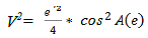
A(e) – azimuth of the geodesic in the Equator
I’n – difference of the Wallis Integrals between b and a, of order n
So:
I’2 = I2b – I2a
I’4 = I4b – I4a
I’6 = I6b – I6a
And from the Wallis Integrals, and limiting to the sixth order:
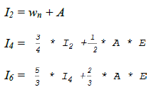
Where:
A = -sin wn * cos wn
E = sin2 wn
For differentiating the difference of distances, we use the distance from the first approximation from the polar triangle of the Figure 1, with the well known formula for w’:
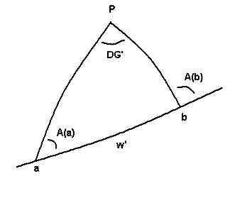
cos w’ = sin L'(a) * sin L'(b) + cos L'(a) * cos L'(b) * cos DG’ … (9)
Where:
w’ – first approximation of the distance s
DG’ – difference of the longitudes [G'(b) – G'(a)]
The formula (9) is not appropriate to compute the correct value for w’ in the remaining calculus because it does not have the accuracy in the case of a small difference of distances. However, it can be used for obtaining the differential of the distance for the Variation of Coordinate’s method.
To obtain the two azimuths A(a) and A(b) and the first correct approximation for w’ as being valid for any distance, the Delambre formulas give an excellent precision in all cases (Pasquay,1972):




Where:
L'(m)– mean latitude is:

DL’– difference of latitudes: [L’(b) – L’(a)]
A(m)– mean azimuth is:

DA – difference of azimuths: [A(b) – A(a)]
We have then:

and

A(a) and A(b) are obtained and also a precise value of w’ for any geodesic, through:

For instance:
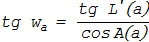
and

(10)
To obtain the azimuth in the Equator, use the Clairaut’s equation (5), where cos L’ = 1:
sin A(e) = sin A(a) * cos L'(a) = sin A(b) * cos L'(b)
And from equation (10):

(11)
Finally, p from equation (4), is obtained by the integration from a to b along the great circle of the sphere with the formula:

once

And from Clairaut’s equation for any latitude L’:
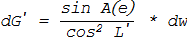
We have then:
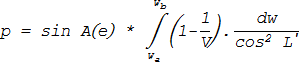
and

and
sin L’ = sin wn * cos A(e)
Limiting the computation to the sixth order, the integration from wa to wb gives:


Taking the flattening:
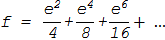
And also:
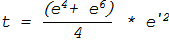
We get finally:
p = sin A(e) * (f * w’ – t * V2 * I’2) (12)
This value is going to correct the value of DG’ in the formula (4). The iterative process continues until we have a difference between two consecutive steps lower than a certain value pre-defined (0.5-14 radians in this case). Then, the process stops and the distance is obtained through formula (8) with an accuracy of an order of a few meters, depending on the angle of the geodesic with the Equator.
Now, we can get the differential of the distance for the observation equation (2). Differentiating (9) relative to L’ and G’ with D = w’ for any station (f), we can have for instance for the station (a) of the system:
-sin D*dD= sin L'(a)*cos L'(f)*dL’- cos L'(a)*sin L'(f) *cos DG’ *dL’- cos L'(a)*cos L'(f)*sin DG’ *dG’
or:


For an OMEGA differential station, we obtain a differential of distances and so, a formula function of the two unknowns dL’ and dG’. Including this formula into the observation equation (2), we have for each series of 3 readings, three equations with two unknowns and through resolution and compensation by the least squares method, we have for each observed set of readings, the two values dL’ and dG’. These are added to the spherical coordinates to obtain the corresponding observed values for (fo):
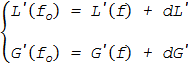
Spherical coordinates are obtained by resolving the equations which must be transformed through appropriate formulas to obtain geographic coordinates. For a statistical treatment, geographic coordinates are not practical and it is much easier to work in rectangular coordinates.
The geographic coordinates are converted to their UTM rectangular coordinates for the remaining steps and the results were traced in a plotter or in a compatible graphical monitor. As the readings are not exempt of perturbations from propagation and other error sources, we obtain a cloud of points that represent the Scatter Plot for each station. With the statistical treatment, a dispersion ellipse with a certain confidence level and other relevant information is determined.
For the calculated points, monthly, mean, covariance σxy, and the standard deviation for the coordinates X and Y (σx and σy) were computed. The dispersion ellipse was also computed with a confidence level of 95%, with its center in the mean point, similar to the method used in topography and triangulation methods (Mikhail and Gracie, 1981) and (Fiadeiro, 1989).
The computed distance and azimuth of the mean position of the OMEGA differential station indicated that a correction to the station was necessary. From the observations, further statistics were calculated and presented in a relative frequency histogram grouped into frequency ranges of distances from each observation to the station, the minimum and maximum distances and the normal or standard deviation.
3. Software
The processing software was written by the author in ANSI FORTRAN 77. It is easy to use, as it is auto learning and can process files already recorded or perform new computations. Data is saved in a file that can be used later for longer periods to compensate for seasonal variations. All OMEGA stations coordinates are included, along with their bandwidths which are used to weight the observation equations to improve the accuracy. Scale is set automatically to plot the results.
The software’s subroutines compute the coordinate transformations both ways, prints the results, executes repetitive computations and matrix resolutions. Dates are converted into Julian Days, for a later use. The graphic output can be directed to a graphical monitor or to a plotter.
The software was written to run on the HP 1000/A900 system of the Hydrographic Institute, with a HP 7550 plotter, a color graphical monitor HP 2397-A Tektronix compatible, or a black and white graphical monitor Tektronix – such was the equipments at that time.
Figure 2 shows the errors for the Porto Santo station, with the corrections that were broadcast to navigators.
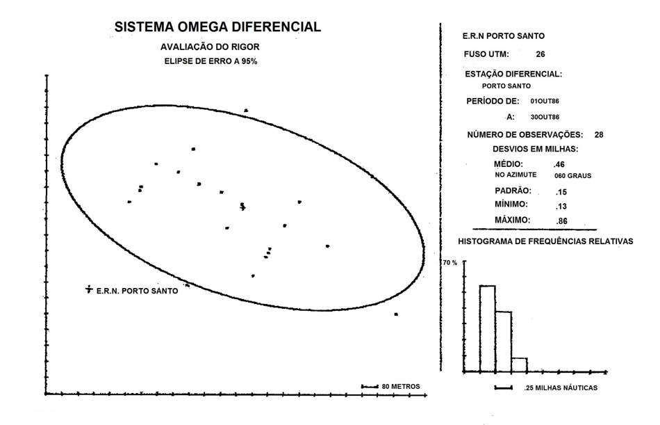
Figure 2 shows the position of the Radio – Naval Station of Porto Santo and also the position of the center of the error ellipse (mean point). The error ellipse indicates the magnitude and the azimuth error of the OMEGA corrections that were broadcast from the station and consequently reported by the users as being faulty. Other information displayed with the plot includes the mean, maximum and minimum values, the standard deviation in nautical miles and a plot of the relative frequency distribution with frequency ranges automatically chosen by the software.
4. Conclusions
This investigation revealed a significant difference in the position of the OMEGA differential station of Porto Santo (approximately half a mile in the azimuth of 60 degrees). The anomaly was corrected and the updated position broadcast. The statistical analysis confirmed normal positional tolerances for the other two stations and did not require any adjustment to their position broadcasts. The measurement results were consistent all year and with expected values for the conditions of the stations – either from the distances between the OMEGA stations, propagation factors or other environmental factors that affect the OMEGA positioning solution.
5. References
Fiadeiro, P. (1989), Complementos de Geodesia, Instituto Hidrográfico, Lisboa, 3a. Edição.
Mikhail, E.M. and Van Gracie, G. (1981), Analysis and Adjustment of Survey Measurements, Nostrand Reinhold Company, New York.
Pasquay, J.N. (1972), Géodésie – Traitement mathématique des mesures géodésiques, ENSTA, Paris, 1972.
Rapp, R.H. (1981), Geometric Geodesy – Vol II (Advanced Techniques), Ohio State University, Columbus.
6. Biography
Pedro Fiadeiro having retired as a Captain in the Portuguese Navy in 1995, Pedro is a consultant on oceanographic and hydrographic studies specialising in statistics and operations research. Educated as Ingénieur ENSTA – Environnement Marin (École Nationale Supérieure de Techniques Avancées), Paris, France. He has a long career in hydrography with surveys along the Portuguese coast and the Azores Islands during the mid-1970s and early 1980s. Other work has included extensive studies of port structure and coastal engineering. He has been the chair of several technical working groups and various senior roles with the Hydrographic Institute including Directorships from 1983 to 1990 and Professor roles with the Naval Academy between 1983 to 1985 and the 1990 to 1995. In these roles, Pedro instigated hydrographic courses that were approved as FIG/IHO Category A and Category B respectively. Between 1998 and 2000, he was the Director of the Earth Environment Agency of the United Earth Alliance.
He has 35 papers published and three books, including 3 articles in the International Hydrographic Review (IHR). He is a full member of the Portuguese Order of Engineers. pfiadeiro@mail.telepac.pt