


Abstract
1. Introduction
Since the development of satellite based positioning, scientists have been striving to increase their derived positional accuracy. There are several error sources that make this difficult: satellite and receiver clock biases; satellite orbital errors; atmospheric delays; multipath signals; bad satellite geometry (GDOP); and measurement noise (Zinas, 2011). The largest uncertainty comes from satellite clock drift, because that causes large uncertainty in phase and code signals. For example, a clock error of 1 µs translates to 300 m in range error (Teunissen and Kleusberg, 1998). This error can be accounted for by double differencing the phase ambiguities between two receivers (kinematic positioning) and can be done in real time (RTK) and post-collection (PPK).
Orbital errors are monitored by international agencies such as the International GNSS Service. Estimates can be provided in real time, but the accuracy is only as good as 5 cm (IGS, 2006). According to Teunissen and Kleusberg’s (1998) simple orbital equation:

satellite orbit errors (dr) are negligible for kinematic techniques as long as the baseline (b) between the receiver and base station is small when compared to the high altitude of the satellites (r). The propagated error (db) will be negligible as long as the baseline is less than 20 km. Even for a 300 km baseline, the largest orbital error would be ~2 cm.
Atmospheric delays are always changing, depending on the state of the Ionosphere and Troposphere (changes in water vapor content and pollution) (Adegoke and Onasanya, 2008). With the introduction of L1 and L2 carrier phase signals, most of the ionospheric delays are eliminated in real time. The two uncertainties that cannot be eliminated with the double difference technique are multi-path and measurement noise. However, multi-path can be limited by choosing good locations surrounded by non-reflective surfaces and by using receivers designed to limit multi-path. Measurement noise is any noise caused by previously unaccounted for uncertainties and electrical noise from the receiver.
Another factor that affects positional accuracy is the satellite geometries relative to the receivers, called Dilution of Precisions, or DOPs. Geometry Dilution of Precisions (GDOPs) will change with time, as satellites move relative to the receiver’s zenith position on earth, and can be broken down into more specific DOPs such a Horizontal and Vertical DOPs (HDOP and VDOP). As satellites move below the horizon, or some set elevation mask, slips in carrier phase cycle can occur and seriously increase positional uncertainty. The introduction of GNSS capable receivers, which allow more satellites such as GLONASS, Galileo, and Compass to be seen, is one way of limiting these errors. Another method to minimize GDOP error is to plan surveys at times when there is good satellite coverage in the area.
To determine how uncertainties in position from RTK, PPK, and RTN methods affect ellipsoid referenced multibeam survey repeatability, bathymetric surveys were conducted on three different days with different GDOP and atmospheric conditions. Soundings from an Edgetech 4600 with different GNSS positional sources were compared to determine the uncertainty and repeatability of a survey with different GNSS techniques. Precise Point Positioning (PPP) GPS solutions were also examined to see how a non- kinematic, non-GNSS post processing technique compares.
There are two types of kinematic solutions, Fixed and Float. Float RTK is an initial estimate of the ambiguity integers. In this status, the rover is essentially creating a grid around itself and going through every single integer possibility until one meets a certain statistical criteria and locks or “fixes” on that solution. A fixed integer solution brings the uncertainty to a centimeter level, which differs from the decimeter level uncertainty of a float status. A minimum of five satellites are needed to do this (Trimble, 2003). Six or more are needed to have the best fixed solution, especially when you have moving baselines.
2. Background
I. PPK and RTK
This project used two GNSS Topcon GR3 receivers to collect PPK and RTK data. The base station receiver was setup on a nearby coordinated benchmark and used a UHF radio link to broadcast RTK corrections to the roving receiver. Post-processing of the GNSS data was conducted with a forward and reverse iteration to achieve the best ambiguity fix possible. This method could be used for any GNSS receiver as long as there is a reference station within a relatively short baseline from the receiver (such as a Continuous Operating Reference Station (CORS)).
II. Network RTK (RTN or NRTK)
Network RTK solutions are able to resolve and predict errors for a large area using a network of reference stations, reducing errors significantly more than a single reference station approach (Zinas, 2011). This widens the range of baselines to 50 -70 km while still remaining within 1-sigma RTK accuracy at the cm level and achieving decimetre level accuracy up to 200 km (Rizos and Han, 2003). Carrier phase ambiguities must be resolved between each of the reference stations in the network and stay resolved at all times through two way communications between stations, usually over the internet. All data is broadcast to a central server that a user can log into and, through one-way or two-way communication, receive the corrections for a Virtual Reference Station (VRS). Zinas (2011) explains, “The receiver sends a NMEA string to the central server and Algorithms at this server generate carrier phase and pseudorange observables for the approximate position using either atmospheric models or regional derived corrections. The virtual observations are then sent back to the user and a single baseline is established with the VRS” (Figure 1). Baselines from the VRS can be up to 70 km, but it is preferred to update your VRS position if you are traveling farther than 20 km.

3. Methods
I. Collection
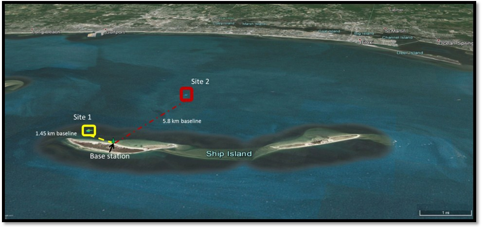
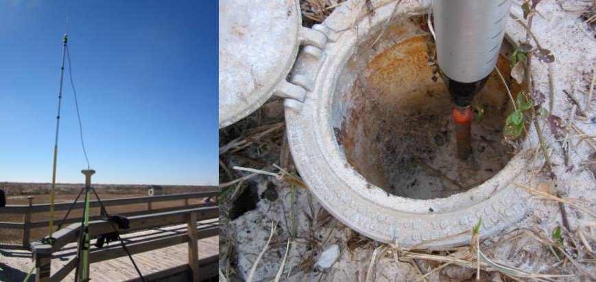
Hydrographic surveys were conducted on three different days: November 26th 2014, January 27th 2015, and February 10th 2015. Survey areas were located in the Mississippi Sound in close proximity to Ship Island, shown in Figure 2. These areas were selected because of the known targets they contain and their proximity to Ship Island, where the RTK base station was established on a recently surveyed benchmark (Figure 3). For quality control, a 4+ hour static observation was done on the benchmark and was post-processed using OPUS (OPUS-RS, 2014) to verify benchmark coordinates.
Two sites were chosen for data collection (Figure 2). Site 1 contained a shipwreck with a 1.45 km baseline to the RTK base station. Two surveys were conducted at Site 1 on 11/26 and 01/27. This site was abandoned for Site 2, which contained larger and more defined targets. Site 2, which consists of an artificial reef made up of concrete culverts and other large rubble, was surveyed once on 01/27 and twice on 02/10. It had a baseline of 5.8 km.
An EdgeTech 4600 bathymetric sonar was used for bathymetry collection, with an Applanix POS MV for real-time navigation and attitude data. The POS MV was supplemented by the GNSS RTN source. RTK and PPK data were collected with two GNSS enabled Topcon GR3’s with UHF radio modems for RTK radio link connections. Data from a Trimble NetRS GPS receiver was also used for a PPP solution.
Gulf Coast Geospatial Center (GCGC) RTN Network (Mississippi’s networked reference stations) corrections were obtained through a cellular AT&T hotspot connection with open source software used to transport RTCM data over the internet (NTRIP) (Lefebure, 2015). HYPACK was used for navigation and line planning. EdgeTech data was collected in Discover, EdgeTech’s proprietary collection software. The LeMoyne, the University of Southern Mississippi’s 29 ft. survey vessel, was the data collection platform.
II. Processing
CARIS HIPS and SIPS 9.0.6 were used for bathymetric and navigation processing. Sound velocity and delayed heave were applied to the data, which was cleaned by the same technician for consistency. A GPS Tide was computed using the GNSS heights (GPS heights for PPP) and applied to reduce the soundings to the WGS84 ellipsoid. The data was then gridded to a 0.5 m surface. This process was done for each navigation source.
Finally, surfaces from two different GNSS kinematic techniques were differenced and compared statistically. MATLAB was used to compare vertical and horizontal differences from RTK, RTN, PPK, and PPP data for each survey. Waypoint’s GravNav was used for PPK processing, plots, and statistics from PPK data.
4. Results/Discussion
I. GNSS
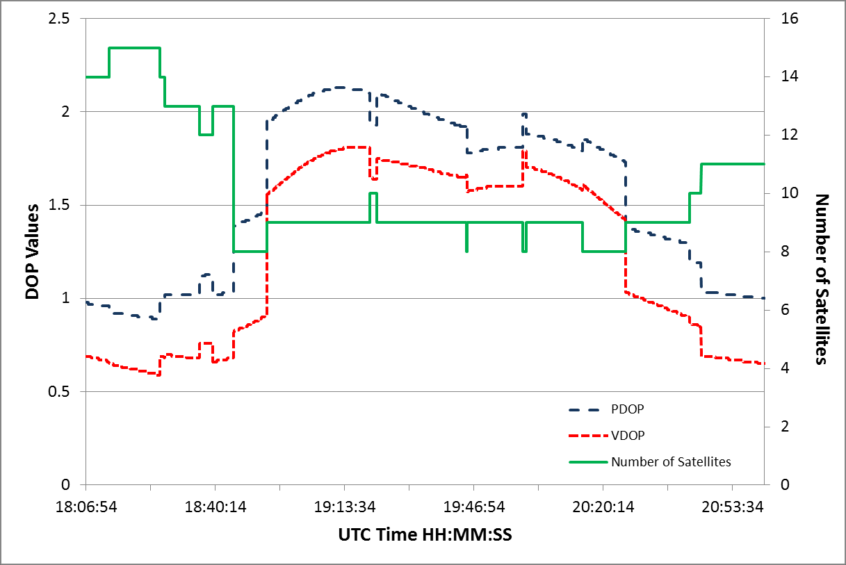
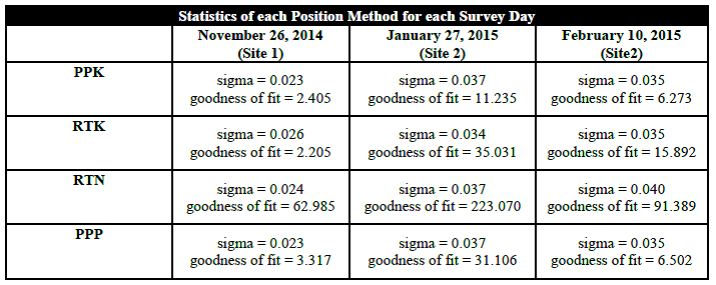
Three survey days were conducted to show the effects of varying GDOPs and how they might affect the data. Table 1 shows how DOP’s (Horizontal DOP (HDOP), Vertical DOP (VDOP), and Positional DOP (PDOP)) vary, throughout and between each survey day. Low DOP values (usually less than 2) are considered optimum (Langley, 2009). The effect of changing DOP values can be seen in a comparison between DOP’s and the number of satellites tracked in Figure 4. An inverse relationship is observed between a drop in the number of satellites being tracked and the DOP increase. Linear regression analyses were run on all vertical GNSS/GPS data for each survey day and sigma values were computed, as well as best-fit residuals (Table 2). These statistics were used as the main determination on which solution had the least uncertainty. The PPK solution had the lowest average sigma value and goodness of fit value over all three days and was used as the navigation source for the control base surface for data comparison. Based on DOP values, February 10th was determined to be the day with least uncertainty in positional data and was used for comparisons of other GNSS data.

Figures 5-7 show vertical positions from each GNSS source for each survey day. The RTN solution has large lapses in time and ellipsoid height, either from cycle slips or cellular internet drop-outs. It is also possible that these lapses occur because we are surveying outside of the RTN network. There are only three reference stations near the survey sites and none on the south side of the survey (Figure 8). The closest reference station is near Gulfport, MS, located 18 and 15 km away from the first and second survey areas, respectively. The other reference stations are 30-36 km away. This is well within the acceptable ranges for network RTK baselines for sub-decimeter accuracy. However, surveying outside the reference station network grid potentially causes triangulation issues in the algorithm and interpolation of the VRS (Wei et al., 2006). This could result in larger positional uncertainty. Horizontal ambiguities need only three reference stations in the area to be resolved, while vertical ambiguities may need up to five, which may result in large vertical uncertainty (Wei et al., 2006). Instances can be seen where the RTK loses its fixed ambiguities or misses a cycle, causing signal drop outs that result in short temporal vertical uncertainty lapses. Post processing RTK data to obtain a PPK solution eliminated these errors and others that were previously unaccounted for.
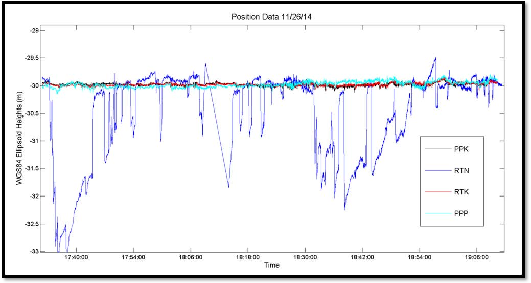
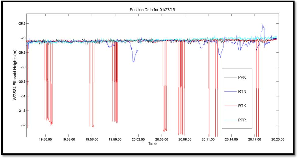

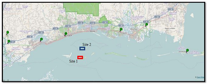
and the blue rectangle is Site 2.
II. Bathymetry
Bathymetric data was processed with data from each GNSS method and gridded to a 0.5 m surface. These were then differenced against the PPK 0.5m surface (Figure 9). Difference surfaces show minimum propagated GNSS uncertainty between methods on a flat sea bed, but a range of differences can be seen around targets on the sea floor. This might be attributed to the EdgeTech 4600’s bottom detection algorithm picking different target points.

Large uncertainties in GNSS data from February 10th do not propagate enough to significantly affect bathymetric measurements. Table 3 shows the significant depth differences calculated from the difference surfaces. To determine the significance of the difference surfaces, the International Hydrographic Organization (IHO) S-44 specifications (IHO, 2008) were used. For Site 2, having an average depth of 5 meters, the maximum allowable THU is 2 meters for a Special Order Survey and 5.25 meters for an Order 1A survey. The maximum allowable TVU for this site was 0.253 meter for Special Order and 0.504 meter for Order 1A (Table 4). Survey data from February 10th had minimal uncertainty and met all IHO specifications for TVU and THU.
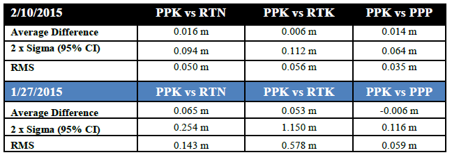
Differences for Jan 27th show large uncertainties in vertical position due to GNSS propagated uncertainty. IHO Special Order TVU accuracies are not met for RTN or RTK positions. This is attributed to the high DOP’s on this day. PDOP’s and VDOP’s spiked to over 4.5 multiple times during the survey as satellites traveled below the set 7 degree elevation mask. Post processing (PPK and PPP) techniques were able to account for the lost ambiguities fixes to meet Special Order requirements.
To test the repeatability of these surveys, 0.5m gridded difference surfaces were made for the second survey site comparing the same GNSS methods from Jan 27th and Feb 10th (Figure 10). Due to previously discussed uncertainties in RTN and RTK data (mainly on the 01/27/15), large differences can be seen when comparing the two survey days. Neither of these methods met IHO Special Order requirements for all soundings on Jan 27th, making them unreliable methods for survey repeatability. The RTK surface has some areas which also didn’t meet IHO Order 1A. However, post processing fixed ambiguities allowing PPK and PPP solutions to meet Special Order criteria for 95% of the Jan 27th survey (Figure 11).


Table 4. IHO Standards for Hydrographic Survey (S- 44) (van Norden, et al, 1998). The 95% Confidence Levels are calculated by:  where a and b are given for each order and d is depth (see IHO S -44 for further information).

(01/27/15 and 02/10/15) at Site 2.
5. Conclusion:
Hydrographic surveying is quickly adopting the technique of surveying to the ellipsoid to remove the need for accurate tidal benchmarks in the survey area. This places a heavy dependence on GNSS accuracies. Do current GNSS techniques provide solutions that make this possible and reliable in all conditions? Of the GNSS methods tested in this study, the two post-processed methods (PPK and PPP) are the only reliable methods when faced with varying DOP’s, increasing baselines, and internet outages (for RTN) for the Mississippi Sound area. RTK performed well for days where DOP’s were good and having greater than 8 satellites for the majority of the survey. However, it could not keep from losing ambiguity fixes due to a change in DOP with baselines larger than 3 km. RTN uncertainty propagation was better than expected. Being outside of the GCGC RTN network geometry was predicted to be a larger source of uncertainty, but it is believed that internet service through the AT&T hotspot was the main reason for high uncertainty in the RTN solution. However, this theory has not been tested and would require further study.
Ellipsoid referenced surveys in this area are recommended to use post-processed data. This ensures repeatable surveys with low uncertainties. For the Mississippi area, real time kinematic GNSS methods are not efficient enough to provide high accuracy repeatable swath bathymetric surveys with baselines larger than 3 km. This could also be the case in other coastal areas similar to the Gulf Coast. To achieve real time kinematic efficiency, networked RTK reference stations and additional cell towers should be set up on barrier island systems. This would ensure good internet coverage as well as good signal geometry for RTN corrections. These factors would allow hydrographers to reliably achieve GNSS sub-decimeter uncertainty in real time anywhere in the Sound, eliminating the need for post-processing.
6. References:
Adegoke, A.S., M.A. Onasanya M.A. “Effects of Propagation Delay on Signal Transmission.” The Pacific Journal of Science and Technology 9.1 (2008): 13-19. The Pacific Journal of Science and Technology, © 2004-2014. Akamai University, Hilo, HI, U.S.A. Web. 1 Mar. 2015. <http://www.akamaiuniversity.us/PJST.htm>.
“IGS — International GNSS Service.” IGS — International GNSS Service. International GPS Service, 12 June 2006. Web. 1 Mar. 2015. http://igscb.jpl.nasa.gov/
IHO, (2008). IHO Standards for Hydrographic Surveys (S-44), Ed. 5, Feb 2008, International Hydrographic Organization, Monaco.
Langely, R.B. “Dilution of Precision.” GPS World 20.5 (2009): 52-59. Iastate.edu. GPSWorld. Web. 24 Apr. 2015. <http://www.nrem.iastate.edu/class/assets/nrem446_546/week3/Dilution_of_Precision.pdf>.
Lefebure (2015). NTRIP Client | Lefebure. Lefebure Design, LLC, 2015. Web. 4 Mar. 2015., <http://lefebure.com/software/ntrpclient/>
OPUS-RS. (2014). KKC OPUS-RS version 1.95
Rizos C., Han S. (2003). Reference Station Network Based RTK Systems – Concepts and Progress. WUJNS. Vol. 8 No.2B, pp.566-574. DOI: 1007-1202(2003)02B-0566-09.
Teunissen P.J.G., Kleusberg A. (1998). GPS for Geodesy. 2nd Edition, Springer, Germany.
Trimble (2003). Real-Time Kinematic Surveying, Training Guide. Part Number 33142-40 Revision D, September 2003.
Van Norden, Max F., Elliot N. Arroyo-Suarez, and Arthur S. Najjar. “Hydrographic Surveys to IHO Standards without Shore Stations using the Real-Time GIPSY (RTG) Global Positioning System (GPS).” NAVOCEANO Product
Wei, E., H. Chai, Z. An, and J. Liu. “VRS Virtual Observations Generation Algorithm.” Journal of Global Positioning Systems J. of GPS 5.1-2 (2006): 76-81. Web. 2 May 2015. <http://www.gnss.com.au/JoGPS/v5n12/v5n12p13.pdf>.
Zinas, Nicholas. “Tekmon Geomatics.” Tekmon Geomatics. 1 Jan. 2011. Web. 1 Mar. 2015. <http://www.tekmon.eu/>.
6. Biographies
Christopher McHugh
Christopher McHugh received his Bachelor’s degree in Marine Science from Coastal Carolina University. He recently graduated with his Masters in Hydrographic Science with an IHO Category A Certification from the University of Southern Mississippi. Christopher has worked for the USGS; Lamont Doherty Earth Observatory onboard the RV Marcus G. Langseth; Burroughs and Chaplin Center for Marine and Wetland Science; and the RBA group. Currently he is working as a Hydrographic Technician at Terrasond Limited.
Ian Church
Ian Church recently completed his PhD in Geodesy and Geomatics Engineering with the Ocean Mapping Group at the University of New Brunswick. He is now working as an Assistant Professor within the Department of Marine Science at the University of Southern Mississippi. His research focuses on using multibeam sonar to improve the understanding of coastal ecology and using 3D hydrodynamic modelling to aid hydrographic data processing.
David Maggio
David Maggio recently graduated from the University of Southern Mississippi’s Department of Marine Science with a Masters Degree in Hydrographic Science and IHO Category A Certification. He is currently employed with TerraSond Limited.
Min Sung Kim
Min Sung Kim completed his bachelor’s degree in Marine Science from the University of the South Pacific. He recently obtained a Master’s in Hydrographic Science and IHO Category A Certification from the University of Southern Mississippi. He currently works as a Hydrographic Technician at Terrasond Limited.