


Abstract
Introduction
During offshore site investigations such as seabed mapping and subsea infrastructures inspection campaigns, hydrographic survey contractors mainly use two types of hydrographic survey systems: surface and underwater systems. In preparing for these survey operations, the contractor needs to estimate the error budget of the hydrographic survey systems to be used. The knowledge of the error budget has many interests:
- To ensure that the procedures and equipment used will meet the survey specifications required of the client. These specifications should align with the IHO’s S-44 standards (IHO 2008);
- Identify and correct errors (random and systematic) during data processing;
- Automatically clean a dataset via the algorithm CUBE developed by Calder (2003).
The objective of this paper is to analyze the predictive error budget – called the “error budget or Total Propagated Uncertainty (TPU)” – for surface and underwater survey systems, and to propose new algorithms to estimate it.
This paper is organized in three parts. Part 1 presents a detailed description of a hydrographic survey system, defines the reference frames and transformations and finally, introduces the concept of error budget. Part 2 presents an error budget estimation method and includes the derivation of the equations of a sounding position acquired by each type of hydrographic survey system. Finally, Part 3 is devoted to the implementation of the error budget estimation algorithms. The validation of the underwater system estimator was done using data acquired during deep water pipeline inspection by an AUV on behalf of the oil and gas company TOTAL.
Part 1. Problem Statement
1.1 Description of hydrographic survey systems
1.1.1 Surface survey system
Classically, a surface survey system is composed of several sensors: a sound velocity probe (SVP), a GNSS positioning system, a motion sensor (Inertial Motion Unit – IMU / Inertial Navigation System – INS and a gyrocompass) and a Multi-Beam Echo Sounder (MBES), all mounted on a vessel (Figure 1). The MBES measures the water depth. The SVP is used to determine the sound velocity profile in the water column in order to correct the depth measured by the MBES from sound speed variations. The IMU measures the vessel attitude. Using the GNSS it is possible to calculate the vessel position. The heave sensor measures the vessel heave.
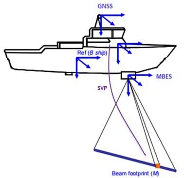
However, each sensor acquires its data in its own frame. The multiplicity of frames is a source of error. Frames of sensors, among others the IMU and MBES frames, need to be aligned (Debese 2013) for data processing. As much as possible, the alignment of the sensors is achieved during the system installation. Possible misalignments between sensors are generally corrected during the classical patch test calibration method or by automatic calibration methods (Seube 2014). Furthermore, data from the various sensors are not acquired exactly at the same time. Latency between sensors is taken into account.
1.1.2 Underwater survey system
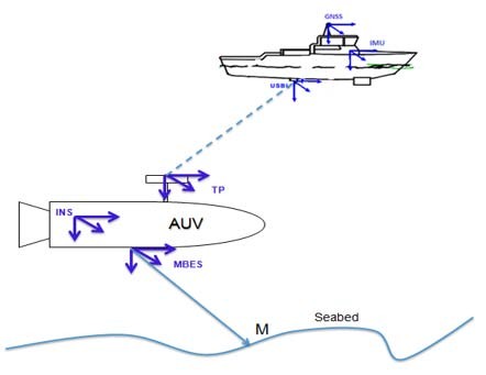
The underwater survey systems are commonly used to provide high resolution data for deep water offshore projects (depth > 100m). Figure 2 illustrates the various sensors and frames of an underwater survey system. Possible misalignments between the sensors are also encountered in these systems and corrected during the calibration phase. For more details on classical calibration methods of an underwater positioning system, see Skilltrade (2012).
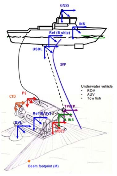
An underwater survey system is composed of a mother vessel at the surface and an underwater vehicle which are positioned relatively to an underwater acoustic positioning system (Ultra-short baseline – USBL). The underwater vehicles generally used are:
- AUV (Autonomous Underwater Vehicle)
- ROV (Remotely Operated Vehicle)
- Tow fish
Underwater vehicles are generally fitted with a number of oceanographic sensors. Their navigation system is based on an INS which takes angular rates and specific forces from the IMU as inputs. Based on an initial acoustic position, the INS calculates the vehicle position, attitude and velocity. A pure inertial solution will drift off rapidly with time. Navigation aiding can be performed using a wide range of sensors such as Doppler Velocity Log (DVL), acoustic positioning system (USBL), and pressure sensor. Once a suitable aiding framework is established, a Kalman filter (KF) is usually applied when carrying out the data fusion in order to obtain the final vehicle trajectory. An exhaustive description of KF applied in inertial navigation can be found in Seube (2014), Farrell (2008) and Groves (2013).
1.2 References frames and transformation
The purpose of this section is to define the various reference frames and transformations between them to estimate the sounding position equations acquired by a hydrographic survey system. The main frames used are: terrestrial reference frame (TRF), local geodetic frame (LGF), local navigation frame or map projection system, body frame and sensor frame.
1.2.1 Terrestrial reference frame (TRF)
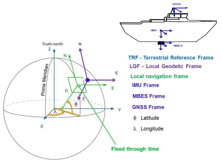
The TRF is an earth-centered earth-fixed (ECEF) frame. Its origin is located at the Earth’s center. Its z-axis points along the Earth’s axis of rotation from the center to the North Pole. The x-axis points from the center to the intersection of the equator with the prime meridian. The y-axis completes the right-handed orthogonal set, pointing from the Earth’s center to the intersection of the equator with the 90° East meridian (see Figure 3).
1.2.2 Local geodetic frame (LGF)
The LGF is used to define the vessel orientation with respect to TRF. It is defined as follows:
- Its origin is located at the IMU frame origin.
- Its x-axis denoted N-Northing, points to true north.
- Its z-axis denoted N-Down, points toward the Earth’s interior, normal to the reference ellipsoid.
- Its y-axis denoted E-Easting, completes the right-handed coordinate system, pointing to east. The x-axis and y-axis lie on the tangent plane to the ellipsoid at the point of interest (see Figure 3).
It should be noticed that when moving relatively to the Earth, the system rotates about its z-axis to allow the x-axis to always point towards the North (Bjørn & Einar 2005).
1.2.3 Local navigation frame
The local navigation frame (projected coordinates system) is used to determine the sounding position. Its axis are defined like the LGF axis, however its origin and orientation are fixed through time at an interest point (see Figure 3).
1.2.4 Body frame (or IMU frame)
The origin of body frame is fixed to the IMU frame origin. The IMU frame is symbolized by (bI). These axes remain fixed with respect to the IMU. The x-axis is defined in the forward direction of the vessel; the z-axis is down axis, pointing in the usual direction of gravity; and the y-axis is the right axis completing the orthogonal set.
1.2.5 Sensor frames
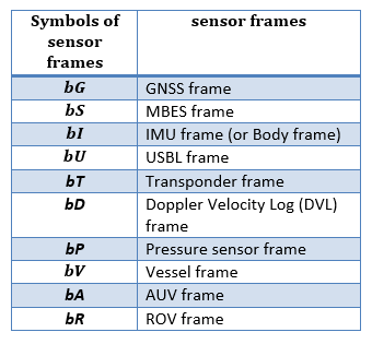
Sensor frames are attached to each sensor of the hydrographic survey system. The symbol b in front of a capital letter is used in this report to represent sensor frames (see Table 1). A sensor frame is commonly defined as follows:
- Its origin is located at the sensor specific point such as the sensor gravity center.
- Its x-axis (roll axis) points towards the forward direction.
- Its y-axis (pitch axis) points towards the right direction.
- Its z-axis (yaw axis) points towards the downward, completing the right-handed coordinate system.
A further reading on the frame definitions and transformations can be found in Seube (2014), Farrell (2008), Debese (2013) and Groves (2013).
1.3 Error budget of an hydrographic survey system
As mentioned in Section 2.1, the sounding position is computed from measurements from the various sensors and procedures. Since the true values of these measurements cannot be determined, it is impossible to determine the exact value of a sounding position and its error. It is however possible to estimate its uncertainty from sounding position equations and the measurement uncertainties associated with each sensor measurement. The purpose of this study is to estimate the measurement uncertainty on the sounding position (N, E, ZDatum) acquired by the underwater and surface survey systems. This is commonly called in hydrography “error budget or Total Propagated Uncertainty (TPU)”.
The TPU is obtained by combining all the error sources contributing to the measurement uncertainty of the sounding position (see Figures 4 and 5) using a statistical method called the uncertainty propagation law in common language the “root-sum-of squares” (JCGM 2008).
Part 2. Proposed method for error budget estimation for hydrographic survey systems
The purpose of this second part is to present a simplified method of error budget estimation for surface and underwater survey systems. The sounding position equations of these systems will be established in order to estimate the error budget of each of hydrographic survey system using the uncertainty propagation law (JCGM 2008).
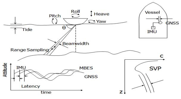
Note that all the errors sources are not illustrated.
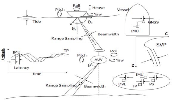
Note that all the errors sources are not illustrated.
2.1 Equations of sounding position of a surface survey system
2.1.1 Geometric description of a surface MBES survey system
As shown in Figure 6, the surface survey system geometry can be described by:
- A reference point which is generally the origin of all lever arm measurements. In this study, the lever arm measurements will be expressed in the body frame.
- Frames attached to each sensor.
- Lever arms. The lever arm measurements between the origin of the frame X and the origin of the frame Y, resolved about the axis of the M frame, denoted bM, are symbolized by
 For instance,
 are the lever arm measurements between the origin of IMU frame and the origin of MBES frame, resolved about the axis of IMU frame.
- A Local Geodetic Frame used to define the vessel orientation with respect to TRF.
- The Terrestrial Reference Frame.
- A Local navigation frame (n) which is the map projection system or mapping frame.
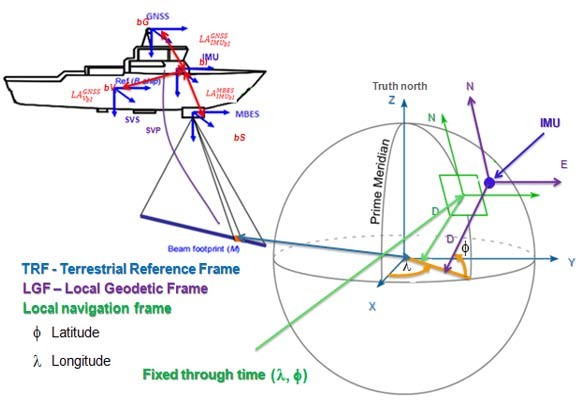
2.1.2 Geo-referencing equations in the local navigation frame
The objective of this section is to determine the equations of a sounding position acquired by a surface survey system in the local navigation frame. This work will establish the equations of a sounding position, first in the MBES frame, then in the IMU frame, the terrestrial reference frame (TRF) and finally in the local navigation frame or map projection frame.
In this paper, the position equations of a sounding will be expressed in the mapping frame coordinate system. These equations will then be derived using a symbolic language tool (Maxima, Matlab, etc.) in order to determine the measurement uncertainty of the sounding position. The approach hypotheses are:
1. The lever arms offsets are already known and resolved about the axis of IMU frame.
2. The misalignments angles between the MBES frame and the IMU frame exist and are known.
3. The sound speed profile of the water column is adequately known.
4. The data acquired by the different sensors of the survey system are synchronous. That is to say that all the sensors measurements are acquired at the same time. However, in reality latency exists between the sensors. The sounding position offset due to the latency effect will be determined in Section 2.1.4.1.
It is important to notice that the most commonly used method in navigation and processing software systems such as CARIS (2004), EIVA, HYPACK, QINSy, etc. for the error budget estimation of a surface survey system was developed by Hare (2001). This approach neglects the covariance between non independent parameters and the latency effect between the IMU and the MBES. They shall be taken into account in this paper.
2.1.2.1 In the MBES frame
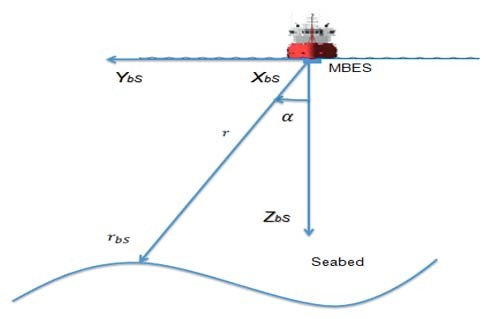
The sounding position coordinated in the MBES frame is obtained from the travel time of the acoustic wave and the incidence angle of beam  . The travel time is converted to slant range r using the speed profile (see Figure 7). The sounding position in the MBES frame can be written as follows. For more detail about the acoustic waves propagation, see (Debese 2013 and Legris 2014).
2.1.2.2 In the IMU frame
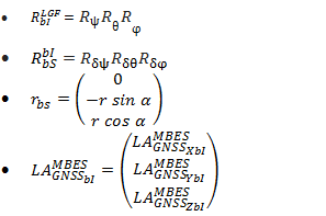
S and I are the origins of MBES and IMU frames, respectively. 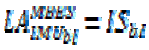 are the lever arm offsets from the origin of the IMU frame to the origin of the MBES frame, coordinated in the IMU frame.
 is the transformation from MBES frame to IMU frame (see Figure 8). The computation of the sounding position (M), in the IMU frame requires two operations:
- A translation for the offsets between the two frames origins,
- A rotation for the misalignment between the two frames.
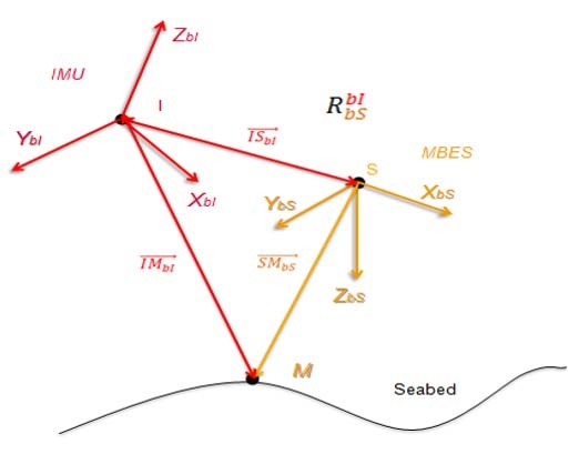
From Figure 8, the sounding position in the IMU frame, denoted 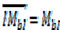 can be written as follows:
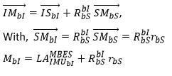
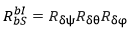
is the transformation matrix from the MBES frame to the IMU frame (boresight matrix). It is described by the misalignment angles (roll misalignment, pitch misalignment and yaw misalignment) between the MBES frame and the IMU frame.
The computation of the boresight matrix is performed into a series of three successive rotations and can be written as below:
2.1.2.3 In the terrestrial reference frame (TRF)
O and P are the origins of TRF and the center phase position of GNSS positioning system, respectively. 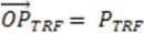 is the phase center position of GNSS in the TRF and
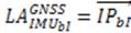 are the lever arm offsets from the IMU frame origin to the phase center position of GNSS in the IMU frame (see Figure 9).
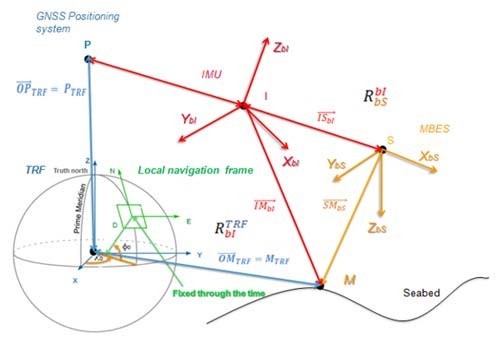
The sounding position denoted  in the TRF, can be written as below:

Therefore, we have:

 is the transformation from the IMU frame to the TRF.

Where:
 is the transformation from the LGF to the TRF;
 is the transformation from the IMU frame to the LGF.
The sounding position in the terrestrial reference frame (TRF) can be written by:

The sounding position coordinated in the TRF can be converted in the local navigation frame (map projection system) using geodetic conversion formulas. For the error analysis purposes, the sounding position should also be expressed in the local navigation – map projection system. In order to avoid taking into account all the existing geodetic projection formulas, an approximation shall be used.
2.1.2.4 Simplified equations of sounding position in the local navigation frame
Finally, the sounding position is expressed in the local navigation frame or the map projection system. The equation above becomes:

With:
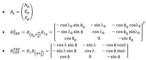
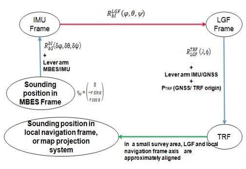
For a relatively limited size survey area close to the origin of local navigation frame  (the local navigation frame is fixed through time), the rotation matrix from the LGF to the local navigation frame (n) can be considered to be the identity matrix. This consideration corresponds to the green arrow shown in Figure 11. This approximation was done to avoid having to consider all the geodetic projection parameters in the following derivation computations.
The equation above becomes:

Where:
 is the phase center position of GNSS positioning system in the local navigation frame. For an ellipsoid referenced survey
 and for a classical hydrographic survey
 ,
 is the transformation from the IMU frame to the LGF which is approximated to the local navigation frame,
 is the sounding position in the MBES frame,
 are the lever arm offsets from the phase center position of GNSS to the origin of the MBES frame in the IMU frame,
 is the sounding position in the local navigation frame.
The simplified equation above can be used for the error budget analysis of a hydrographic survey system. In practice, the lever arms measurements are generally expressed in the IMU frame. In this case, the lever arms measurements are attached to the vessel frame  . It is necessary to express them in the IMU frame as below:

Figure 10 : Summary of the different rotations (in red), transformations (in blue arrow) and approximations (in green) necessary to express the sounding position in the local navigation frame.
2.1.3 Reduction of measured depth acquired by a surface survey system
In hydrography, depths must be referenced to a common vertical datum. Consequently, corrections must be applied to previous position equations in order to get a reduced (or charted) depth. The purpose of this section is to present equations of sounding reduction for two types of classical and ellipsoid referenced surveys.
2.1.3.1 Ellipsoid referenced survey
From Figure 11, the charted depth is described as below:

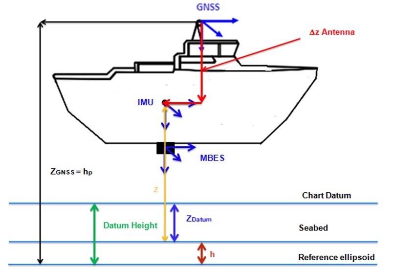
SEP represents the separation model between the ellipsoid and the vertical datum. The absolute sounding position determined by an ellipsoid referenced survey can be given as below:
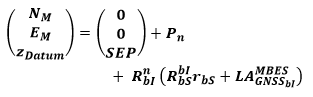
2.1.3.2 Classical hydrographic survey
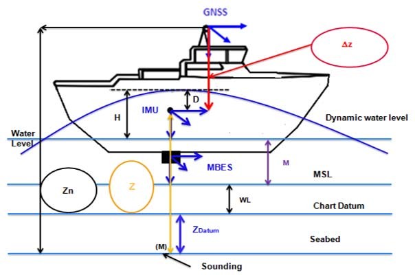
As shown in Figure 12, the charted depth determined by a classical hydrographic survey is given by the formula below:

Where:
- D is the dynamic draft;
- H is the measured heave (Heave sensor);
- M is the measured tide;
- WL is vertical offset between the MSL and the chart datum;
- z is the vertical offset between a sounding located at seabed and the IMU frame origin.
z is equal to the difference between the vertical offset between the seabed and the phase center position of GNSS positioning system, denoted Zn and the vertical offset be- tween the phase center position of the GNSS positioning system and the IMU frame origin denoted  .
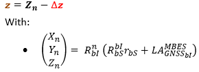
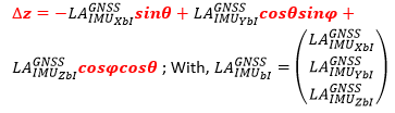
The absolute sounding position acquired by a classical hydrographic survey can be given as follows:

As mentioned in Section 1.1, the data acquired by the sensors of a surface survey system are not synchronous. Latency is introduced between some sensors of the system to take into account the delay for information transmission and computation. This creates a non-negligible offset on the sounding position (Bjørn & Einar 2005). The purpose of the next section is to model the sounding position offset due to the latency.
2.1.4 The dynamic sounding position equations of surface survey system
The mathematical modeling of the sounding position offset due to the latency between the sensors has mainly been studied by Seube (2014) and Bjørn & Einar (2005) in different ways. The proposed approach in this section is based on the approaches of Seube (2014), Farrell (2008) and Bjørn & Einar (2005).
2.1.4.1 Modeling of the sounding position offset due to the latency effects GNSS/MBES and GNSS/IMU
To model the position offset of a sounding due to the latency effect in a surface survey system, we assume that all measurements are subject to time stamp errors apart for the GNSS positioning system.
The time stamp errors of the sensors (GNSS positioning system, IMU and MBES) of surface survey system can be modeled as follows (Bjørn & Einar 2005):
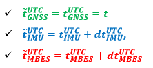
Where  is the sensor time stamp (time recorded by the sensor X),
 is the physical sensor measurement time and
 is the latency between the GNSS positioning system and the sensor X.
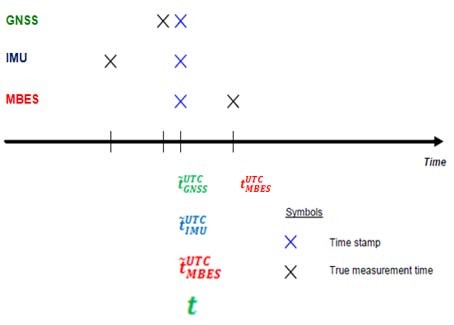
The fake position of a sounding is computed at the MBES time. Indeed the data measured by the IMU and GNSS positioning systems at the instant  and
 respectively, are not the data used to compute the sounding position at MBES time (Figure 13).
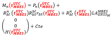
Cte is a vector including the various corrections to determine the charted depth (see Sections 2.1.3.1 and 2.1.3.2).
The final position of a sounding  due to the latency effect in the system can be expressed as follows:
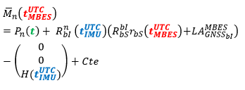
In addition, the measurements can be considered synchronous when deriving the final position of a sounding (Bjørn & Einar, 2005), i.e.  .
The final position of a sounding referred at MBES time becomes:
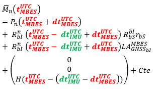
With:

dt is the latency IMU/MBES. It is positive when the physical measurement time of IMU lags behind the physical time of MBES and negative in the opposite case. The sounding position offset  created by the latency effect in the system can be modeled by computing the difference between the final sounding position and
 the fake sounding position at the time
 .
The sounding position offset due to the latency effect in a surface survey system is given as follows:
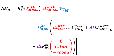
Where:
- the vessel speed resolved about the IMU frame axes.
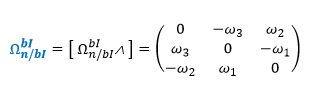
 is denoted the skew-symmetric matrix of rotation angular rate of frame
 with respect to the local navigation frame expressed in the local navigation frame.
This skew-symmetric matrix can be defined as:
The angular rate vector can be expressed in terms of the time derivative of Euler attitudes using (Farrell, 2008):
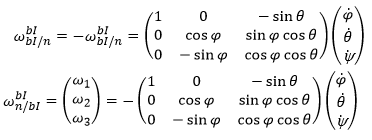
The vessel angular rates are obtained by derivation of attitude data. Finally, the final position of a sounding due to the latency effect can be written as:

2.2 Equations of sounding position for underwater survey system
The purpose of this section is to express the sounding position equations of an underwater survey system in order to estimate its error budget. As mentioned in Section 1.2, an underwater survey system includes a mother vessel and an underwater vehicle such as an ROV, AUV or tow fish. The position of the underwater vehicle is determined by acoustic positioning systems; either via USBL (from the surface) or via a Long Base Line (LBL) network installed under the mother vessel.
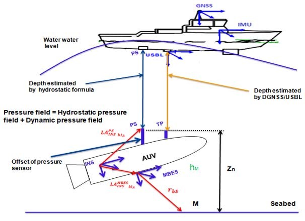
In this paper, we consider a USBL acoustic positioning system (Figure 14), as it is the main system used in the oil and gas industry. The USBL acoustic positioning system delivers ranges and bearings from the acoustic center of an USBL transducer to the transponder (TP) generally located at top side of underwater vehicle.
2.2 Equations for souding position in the navigation frame
The sounding position acquired by an underwater survey system is computed in a similar way to that of a surface survey system. It combines two equations: the transponder position, in the local navigation frame and the sounding position relative to the transponder position, in the local navigation frame.
The transponder position in the local navigation frame can be written as:

And the sounding position in the local navigation frame (n) can be expressed as follows:

Where:
 is the transponder position in the local navigation frame.
 is the GNSS positioning system position in the local navigation frame.
 is the transformation from the USBL frame bU to the IMU frame bIv.
 is the transformation from the IMU frame to the local navigation frame.
 is the transponder position in the USBL frame bU.
 are the lever arm measurements from the transponder frame origin to the GNSS center phase position in the IMU frame, located on the vessel (V).
The sounding position  can be written as function of the AUV position as follows:

Where:
 is the AUV position, in the local navigation frame.
 is the sounding position, in the local gation frame.
 is the transformation from the MBES frame to the INS frame of AUV.
 is the transformation from the INS frame of AUV to the local navigation frame.
 is the sounding position, in the MBES frame.
 are the lever arm measurements from the MBES frame origin to the INS frame origin, resolved about the axis of INS frame, located on the AUV.
2.2.2 Reduction of measured depth
In an underwater surface system, the horizontal position of a sounding is generally estimated by an inertial navigation system integrated in the underwater vehicle, coupled with aiding sensors such as Doppler Velocity Log (DVL), acoustic positioning (USBL) and GNSS positioning (DGNSS/PPP). The charted depth is usually estimated by combining the pressure sensor measurements with the measurement of the water density profile, the tide and atmospheric pressure measurements.
Two sea water density estimation formulas are usually used in the oil and gas industry: the Tritech formula and the UNESCO formula (UNESCO/SCOR/ICES/IAPSO, 1983). These density formulas are empirical formulas. In some parts of the world, the UNESCO formula is more accurate than the Tritech Formula and vice versa. To choose the most appropriate formula for a given survey area, the depth results from the two formulas can be compared with the estimated depth from the USBL transducer.
The traditional formula error depends on many parameters such as the sea density profile, the measurement frequency of the CTD (Conductivity, Temperature and Depth) probe, the numerical integration method used, etc.
The charted depth of a sounding is traditionally estimated by the formula below (Figure 15):

Where:
- hPS is the AUV immersion.
- M is the measured or predicted tide.
- WL is the MSL (Mean Sea Level) height above the chart datum.
- Zn is the vertical offset between the pressure sensor and the sounding located at the seabed.
From (Hagen & Bjørn 2008), the charted depth described by the approach above can be improved by combining the vertical position of the sounding estimated from the hydrostatic formula (UNESCO formula) with the integrated inertial navigation system followed by data post processing.
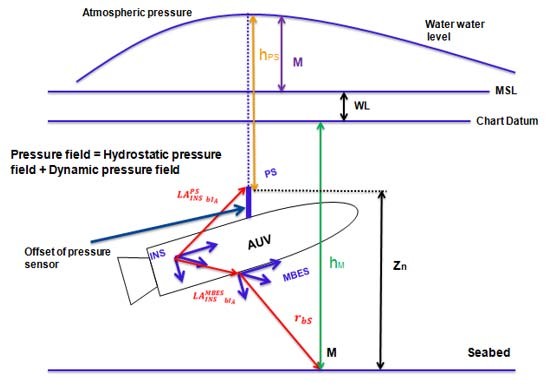
An alternative is to combine a pressure sensor located close to the USBL and the pressure sensor located at the top of the AUV estimated by the hydrostatic formula with the integrated inertial navigation system followed by a post processing on navigation software. It allows discarding the effect of dynamic wave-induced pressure at the sea surface and improves the vertical position of sounding (Figure 16).
2.2.3 Dynamic equations of the sounding position of underwater survey system
To model the sounding position offset due to the latency effect in an underwater survey system, this approach assumes that:
(i) The MBES, IMU, Transponder and USBL are synchronized to UTC time.
(ii) Every sensor produces a perfect measurement, but this measurement is time stamped erroneously, apart for GNSS positioning system.
The time stamp errors of the sensors (GNSS positioning system, IMU and USBL) of surface survey vessel can be expressed as follows:
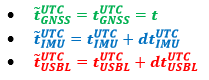
The time stamp errors of the sensors (Transponder, INS and MBES) of the underwater vehicle can be modeled as follows:
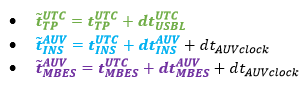
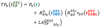
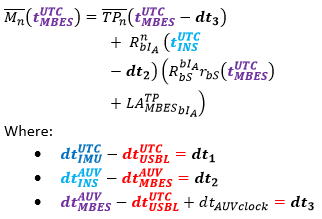
 is the difference between the UTC and AUV time references. For an underwater survey system with an ROV, as all sensors normally remain synchronized to one single time server, should be close to zero. In an AUV survey system, time reference can drift by a magnitude of 50 ms from the vessel time reference when the AUV is submerged (Bjørn & Einar 2005).
(iii) The true position of the transponder is computed at the TP time  follows:
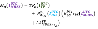
(iv) The true position of the sounding is computed at the MBES time as seen below:
(v) The latency effect between the IMU and the transponder doesn’t affect the heave measurement.
2.2.3.1 Transponder and sounding final positions due to the latency between system sensors
The final positions of the transponder and the sounding due to the latency effect in an underwater survey system are denoted  and
 , respectively and can be expressed as follows: respectively and can be expressed as follows:
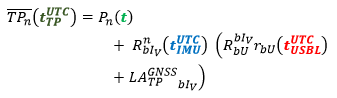
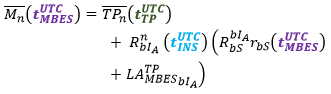
In addition (Bjørn & Einar, 2005) assume that the time stamps are equal (synchronous measurements) when deriving the final positions of transponder and sounding, i.e.:

Then, 
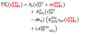
The latency effect on the transponder position has two components. The first is due to time errors in the surface vessel. The second error component is due to the time errors in the underwater vehicle (Bjørn & Einar, 2005).
The final positions of the transponder and the sounding become:
Modeling of the offsets due to the latency effects between the sensors
The transponder position offset  due to the latency effect can be derived in a similar way as in the Section 3.1.3.1 for surface survey systems:
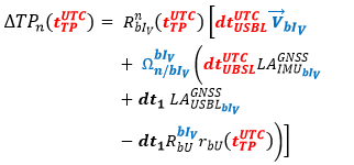
Then the sounding position offset  becomes:
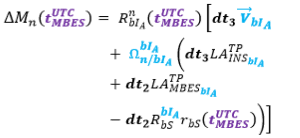
The final position of sounding can be written as:

Knowing the sounding position equations of each type of hydrographic survey system, the purpose of the next section is to estimate their error budget using the uncertainty propagation law (JCGM, 2008).
Part 3. Error budget estimation for hydrographic survey systems
The objective of this section is to estimate the measurement uncertainty of the sounding position acquired by the underwater and the surface survey systems. It will also enable analyzing the effect of each sensor uncertainty on the sounding position accuracy.
3.1 Error budget estimation for surface survey system
The sounding position acquired by a surface survey system depends on several parameters measured by various sensors (MBES, IMU, etc.). Each measurement has an uncertainty. The uncertainties are then combined to estimate the measurement uncertainty of the sounding position by using the law of uncertainty propagation (see Section 2.3).
3.1.1 Algorithm of error budget estimation for surface survey system
The assumptions for the error budget algorithm estimation of the surface survey system are:
1. All the uncertainties of the measurements acquired by the sensors of the system are known. All parameters uncertainties are normally distributed and uncorrelated.
2. The horizontal sounding position uncertainty at 1-sigma  is:

3. The covariance term is in absolute value as it is non negligible. When N and E position coordinates vary in the opposite direction, the covariance term is negative and affects significantly the uncertainty position. This assumption enables having more realistic results.
4. The measurement uncertainty model used for the MBES and the sound speed is the one proposed by Hammerstad (2001).
This algorithm takes into account the covariance between the fake position of a sounding (without latency) and the position offset of the sounding due to the latency effect (or time stamp error) in the system. The partial derivatives of the position equation have been computed with Matlab and imported into VBA (Excel). The following results are obtained:
Figure 17 shows the contributions of each measurement uncertainty of sensors and procedures to the sounding vertical position acquired by ellipsoid referenced MBES survey. The contribution of an uncertainty source is estimated by neglecting the other uncertainty sources. It is clear that the measurement uncertainties of roll and pitch misalignments have a significant influence on the sounding vertical position. They increase with the incidence angle. The latency effect MBES/IMU has a direct impact on the angular rates (more on the roll angular rate which is the major component of skew-symmetric matrix (Farrell 2008). For more details, see Section 3.1.3.1. It can be noticed that the accuracy of an angular rate is approximately equal to the accuracy of its angle.
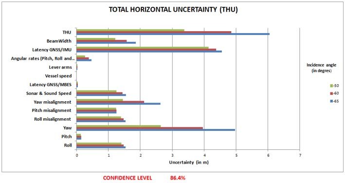
It can be seen that the yaw uncertainty is the major contributor to the total horizontal uncertainty of sounding. Moreover, a very accurate calibration of angle misalignments and latencies (GNSS/IMU and GNSS/MBES) is necessary to significantly improve the total horizontal uncertainty of sounding. Moreover, from Figure 18, the latency in the GNSS/IMU makes a significant contribution to the TVU.
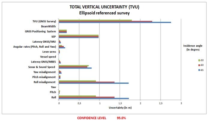
The study of Figures 17 and 18 shows on which sensor, and which parameter, the survey operator should focus on. It clearly appears that an error on the angular rates will have less impact on the sounding accuracy than an error on the yaw for instance. This should be used by hydrographic companies/ services to improve their equipment and procedures.
3.2 Error budget estimation of underwater survey system
The sounding position acquired by an underwater survey system depends on more parameters than a surface survey system does. The measurement uncertainty on the horizontal position is equal to the square root of the sum of variances of the measurement uncertainty of the transponder horizontal position and the measurement uncertainty of the sounding position relative to the transponder position. The measurement uncertainties on the transponder position and the sounding position relative to the transponder are estimated by applying the uncertainty propagation law to their position equations. The vertical position of the sounding is determined in a similar way.
In practice, the transponder position (or underwater vehicle) is usually determined from the acoustic (DGNSS/USBL) and inertial (IMU) positioning methods, as they have complementary qualities. Acoustic positioning is characterized by a relatively high and evenly distributed noise and no drift in the position, while inertial positioning has a very low short-term noise and relatively large position drift over time (Kongsberg, 2015). Data post-processing on navigation software can enhance the measurement uncertainties on transponder position by 50% to 70% (Kongsberg 2015). From iXBlue (2004), the yaw uncertainties could be improved by approximately 50%. The navigation software used both the past and future sensors’ measurements and their un- certainties computed by the Kalman filter.
3.2.1 Algorithm of error budget estimation of underwater survey system
To estimate the measurement uncertainty of sounding position acquired by an underwater survey system, we make the same assumptions than those made for surface survey systems. The following results were obtained:
Figure 19 shows the contributions of each measurement uncertainty of sensors and procedures to the sounding vertical position acquired by an AUV survey. The sonar measurement uncertainty has an important effect at the nadir as shown by the curve of the uncertainty contribution of sounding position relative to the transponder.
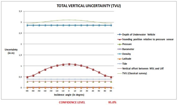
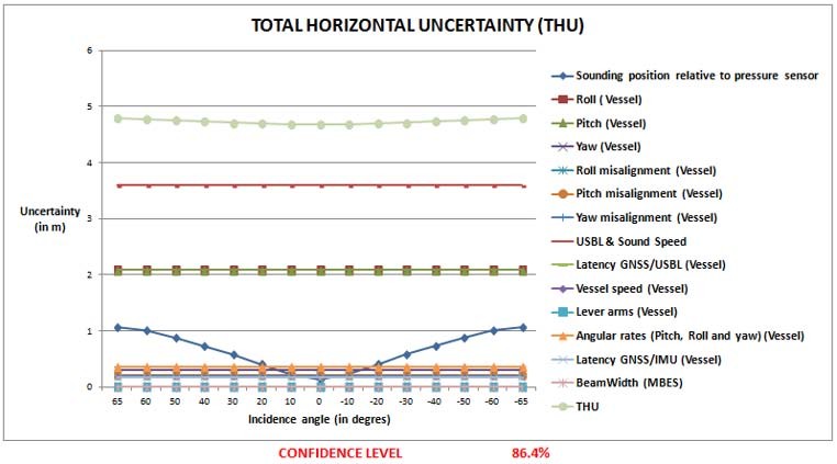
Figure 20 shows the contributions of each measurement uncertainty of sensors and procedures to the horizontal sounding position acquired by a classical AUV survey system. The TVU increases as the sounding moves away from nadir with a magnitude of 6m at 86.4% of confidence level. The TVU is more affected by the measurement uncertainty of roll and can be significantly improved using a very accurate IMU. This argument has been raised by (Kongsberg 2015).
Implementation on pipelines inspection campaign by AUV
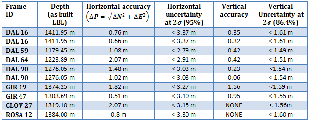
To validate the error budget estimation algorithm for the underwater and surface survey systems described in the previous paragraphs, in 2014, TOTAL conducted an AUV pipeline inspection campaign in Angola. Permanent LBL frames previously located by LBL positioning techniques and least square network adjustment were also measured by a MBES mounted on AUV. The comparison between LBL reference coordinates and those measured by AUV gives an indication of the sounding accuracy. This effective accuracy will then be compared with the TPU estimated using the TPU algorithm. The comparison enabled the validation of the TPU algorithm.
The positions acquired by LBL acoustic positioning technique are taken as reference positions, as a permanent LBL network provides a very high positioning accuracy (Sonardyne 2015). The horizontal uncertainties are generally better than 1m and can reach 10cm. A disadvantage of the system however is its time consuming installation and calibration during offshore operations, which has a commercial impact when deciding on suitable positioning systems (Sonardyne 2015). For more information about, the LBL acoustic positioning technique, see Sonardyne (2015), Groves (2013) and Jong (2013).
Table 2 shows the accuracies of frames positions and the predicted uncertainties of these positions via the error budget estimation algorithm. The depth as-built-LBL is the depth estimated during the LBL frame installation using the traditional formula (mean sea water density). The AUV depth was also estimated using the traditional formula. The measurement uncertainty of the sea water density taken in this study is 0.4 kg/m3.
These results are very satisfactory, as the uncertainties of LBL frames positions are superior to obtained accuracies, but not too different.
Conclusion
The objective of this project was to analyze the error budget for surface and underwater survey systems. The major outcomes of this work can be summarized as follows:
- Improvement of the sounding position acquired by the underwater and surface survey systems.
- Improvement of the error budget estimation algorithm for underwater and surface survey systems. The major added value are:
- – The consideration of the covariance between the coordinates X and Y and the propagation of errors of a functional MBES model.
- – The consideration of latency errors between the sensors of hydrographic survey systems.
- Demonstration that a yaw misalignment between the IMU and the MBES influences the vertical position of sounding.
The main outcome of this study is the implementation of error budget estimation algorithms applied to underwater and surface survey systems. These tools will be used by TOTAL to evaluate the technical aspects of contractor proposals, to better qualify the accuracy of acquired data and to improve their survey methodologies and accuracies.
The error budget estimation and position equations algorithms for underwater and surface survey systems can be easily imported in JAVA, FORTRAN, C and PYTHON in order to quickly update hydrographic data acquisition, navigation and processing soft- wares. An implementation of error budget estimation tool was done on the data of the inspection campaign of pipelines by an AUV with satisfactory results.
Grateful thanks for the members of the hydrographic survey community involved in this project for their insightful and constructive help. This objective could be achieved through the combined efforts of several people of the hydrographic survey community. This paper benefited from comments from: Vincent LATRON (TOTAL), Marie-Laure GEAI (TOTAL), Frederic AUGER (TOTAL), Pierre BOSSER (ENSTA Bretagne), Patricia GASPAR (CARIS), Marc KEBBEL (FUGRO), Nathalie DEBESE (ENSTA Bretagne), Arnaud VIDAL (TOTAL), Chris MALZONE (QPS), Emilie BLANCART (TOTAL), Rabine KEYETIEU (CIDCO), Jeppe NIELSEN (EIVA) and Colin CAMERON (DOF Subsea).
References
Bjørn, J. & Einar, B., 2006. Time Referencing in Offshore Survey Systems.FFI/RAPPORT- 2006/01666, Norwegian Defence Research Establishment.
Calder, B., 2003. Automated Statistical Processing of Multibeam Echosounder Data. International Hydrographic Review, Vol. 4 No. 1, pp. 53-68.
CARIS, 2004. Total Propagated Uncertainty Computation.viewed 20 July 2015, http://www.caris.com/tpu/.
Debese, N., 2013. Bathymétrie. Sondeurs,traitement de données, modèles numériques de terrain. Paris: Ellipses Editions Marketing S.A.
Farrell, J., 2008. Aided Navigation: GPS with High Rate Sensors. New York: McGraw-Hill.
Groves, P. D., 2013. Principles of GNSS, Inertial, and Multisensor Integrated Navigation Systems. Second Edition ed. Houston: Artech House.Hagen, O. K. & Bjorn, 2008. Vertical Position Estimation For Underwater vehicles.
Hammerstad, E, 2001. Multibeam Echo Sounder Accuracy. EM Technical Note, Kongsberg Simrad AS.
Hare, R., 2001. Error Budget Analysis for US NAVAL Oceanographic Office (NAVOCEANO) Hydrographic Survey Systems, Mississippi: University Mississippi.
Hare, R., 2004. CUBE & Navsurface, viewed 1 June 2015, http://www.google.fr/url?url=ftp://moray.dms.usm.edu/archived/cube/8a_Hare%2520on%2520CUBE%2520%26%2520NavSur-face.ppt&rct=j&frm=1&q=&esrc=s&sa=U&ei=PDhsVZ35JZKf7gbb4YDoCQ&ved=0CBQQFjA A&usg=AFQjCNEntKcc6bz-4HFXOyExYWuc5m0TQw.
International Federation of Surveyors (FIG), 2006. FIG Guide on the development of Vertical Reference Surface for Hydrography.
International Hydrographic Organisation (IHO), 2008. S-44 – IHO Standards for Hydrographic Surveys, 5th Ed, Monaco.
iXBlue, 2004. USBL Positioning Systems, Viewed 20 July 2015. http://www.ixblue.com/products/usbl-positioning-systems.
Joint Committee for Guides in Metrology (JCGM), 2008. Evaluation of measurement data – Guide to the expression of uncertainty in measurement.
Jong, K. D., 2013. Offshore Positioning, Brest. Kongsberg. High Presicion Acoustic Positioning – HIPAP, viewed 20 July 2015. http://www.km.kongsberg.com/ks/web/nokbg0397.nsf/AllWeb/ D3F9B693E19302BBC12571B6003DD0AE/$file/HiPAP_Family_brochure_v3_lowres.pdf?OpenElement.
Legris, M., 2014. Cours de bathymétrie à l’ENSTA Bretagne, Brest.
Seube, N., 2014. Cours d’hydrographie à l’ENSTA Bretagne, Brest.
Skilltrade, 2012. Handbook of Offshore Surveying. 2nd Edition, Vol. II.
Sonardyne, 2015, Acoustic positioining. viewed 30 July 2015, http://www.sonardyne.com/products/positioning/lbl.html.
UNESCO/SCOR/ICES/IAPSO, 1983. Algorithms for computation of fundamental properties of seawater.
Biographies
Geraud NAANKEU WATI received his Master I in Mechanical and Numerical Simulation from the University of Maine, Le Mans, France, in 2013 and his Master’s degree in engineering in Hydrography and Oceanography from the ENSTA Bretagne, Brest, France, 2015. In 2015, he completed his final year project at TOTAL E&P, focused on error budget analysis for hydrographic survey systems. He is very motivated to join a survey department or a research center specialized in geodesy, geomatics or oceanography all over the world (Europe, Africa, America, etc.).
Email: wgeraud@yahoo.fr
Jean-Baptiste GELDOF received his Master’s degree in engineering in Topography from the INSA Strasbourg, Strasbourg, France, in 2011. From 2011 to 2012, he was a survey Engineer at IOTA Survey. Since 2012, he is a Geomatic and Positioning engineer at TOTAL E&P. He worked on various offshore survey projects in various countries (Cameroon, Gabon, Nigeria, Azerbaijan, Qatar, etc.). He is mainly focused on geodesy and positioning, topographic and hydrographic surveys and Geographical Information Systems.
Email: jean-baptiste.geldof@total.com
Nicolas SEUBE received his doctorate in applied mathematics from the University of Paris Dauphine, France, in 1992. From 2005 to 2014, he was the Head of the hydrography department at the ENSTA Bretagne, France where he constituted a group instruction and research in hydrography. In 2010, he established a consortium of three universities (ENSTA Bretagne, UGhent (Belgium) and HCU (Germany) and created the Eramus project “Intensive program in Hydrography and Geomatics”. In 2011, he was named as a representative on the FIG/IHO/ICA International Board on Standards of Competence for Hydrographic Surveyors and Nautical Cartographers. He was elected president of this committee in 2013. In 2013, He was awarded the “André Giret” prize for his contribution to the French hydrographic research and education. Since 2014, he has been the scientific director of CIDCO Canada. His recent research focuses on the rigorous approaches of calibration (latency and viewing angles) LIDAR terrestrial mobile systems and the automatic detection of systematic errors in the LIDAR and Multi-beam echo sounder (MBES) data datasets.
Email: nicolas.seuble@cidco.ca