SOUND VELOCITY PROFILE (SVP) INVERSION THROUGH CORRECTING THE TERRAIN DISTORTION

1. Introduction

During multi-beam bathymetric data processing, the speed of sound varies with depth and can cause the oblique sounding ray paths to bend, introducing significant and systematic biases in soundings which leads to terrain distortion. The accuracy of bathymetric survey can be greatly improved by using corrected Sound Velocity Profile (SVP) data.

SVP sampling is the major method of obtaining sound velocity during a multi-beam bathymetric survey. (Herman, et al. 1998). Current survey practice requires that sound velocity measurements are taken near the extreme times of water temperature changes during the day, being 08:00 am, 02:00 pm and 08:00 pm. Rather, it is preferred that sound velocity measurements are taken nearer the time of the bathymetric data collection. (ZHU, 2011). Due to the variability in time and space, the ray trace solutions of multi-beam bathymetry collected using current methods won’t necessarily meet the accuracy requirements for all bathymetric data. Thus, the distortion in the resultant seafloor terrain can be the result of sound velocity differences (errors) between the SVPs. During the multi-beam bathymetric data processing, the terrain distortion caused by sound velocity differences, can be corrected, by adjusting the Coefficients parameter of Refraction in commercial processing software.

Based on the measurement characteristics discussed, mode vectors can be obtained by EOF using real SVPs obtained in the survey area. Correcting the terrain distortion, the inversion result of the SVP can be determined by Genetic Algorithm (GA). Finally, these methods have been tested using observed data.

2. Terrain Distortion Caused by Sound Velocity Errors

Changes in temperature and salinity throughout the water column affect sound velocity. Changes in the physical properties of the medium causes deflection of the acoustic direction. If the ray traced solutions are computed using the incorrect sound velocity profile, the incorrect ray paths will lead to a lower accuracy in the bathymetry measurement and increased terrain distortion. (LI, et al. 1999, DONG, et al. 2007, LI, et al. 2001, ZHAO, LIU 2009).

When the sound velocity at the surface is less than the sound velocity at lower depths, the terrain distortions are concave. Where the above is reversed, the terrain distortions are convex. (DONG, et al. 2007, DONG, et al. 2011). If the adjacent two swaths are both distorted, there is a “ridge” or “groove” in the along-track direction. As shown in Figure 1, both of the multi-beam swaths are concave and there is a “ridge” in the along-track direction. Hence it can be determined that the SVP used to compute the ray traced solutions of the multi-beam bathymetry is wrong in this area.

3. Sound Velocity Profiles (SVPs) by EOF Modeling

A SVP is the vertical distribution of a velocity structure and can be estimated by some regularity in coastal and ocean areas. (Cartwright, 2003, Kammerer, 2000, ZHU, 2011). They can also be described by a parametric model. (ZHANG, et al. 2011). Currently, there are two parametric models for determining SVPs: Analytic Function (AF) and Empirical Orthogonal Function (EOF).

According to LeBlanc and Middleton (1980), it is a valid method to describe the SVP using an EOF parametric model based on the spatio-temporal correlation of the profiles. (DING, et al. 2007, LeBlanc and Middleton, 1980, SHEN, et al. 1999, PENG, et al. 2003, HE, et al. 2006). First, mode vectors via EOF are obtained based on real, measured SVPs. When combined with the sample data, reconstructed modeled SVPs can then be obtained.

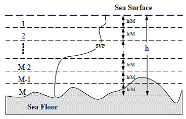
The modeling process follows:

As is shown in Figure 2, N is the number of SVPs in the survey area. Interpolating M equally spaced vertical measurements to a standard floor, the SVP standardization matrix C with a size M x N of can be obtained:

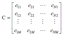
(1)

The average SVP can be obtained after each row of the standardization matrix is averaged.

The SVP disturbance matrix is obtained by subtracting each column C and and is the covariance matrix of the SVPs disturbance matrix . As shown below, the covariance matrix eigenvalue decomposition:

(2)

is the matrix consisting of characteristic values and F is determined from the feature vectors from the matrix R .

(3)

is the eigenvalue corresponding to the feature vector (EOF mode). Thus, each SVP in the survey area can be represented with K dimension vectors:

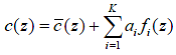
(4)

Where are the coefficients of SVP reconstruction.

Once obtained they are used for inversion of the SVP.

Moving to the left side of the equation (4):

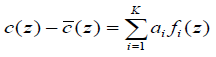
(5)

(6)

According to least squares theory:

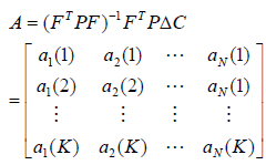
(7)

4. Inversion of the SVP by correcting the terrain distortion

The inversion of the SVP is a method whereby the acoustic properties of the ocean can be estimated by using observed data. Many scholars have proposed methods associated with this problem (HE, et al. 2011, JIN, et al. 1996, Lindsay and Chapman, 1993, Vaccaro, 1998, ZHANG, et al. 2002). This section discusses how mode vectors obtained via EOF are used for the inversion of the SVP. By correcting the terrain distortion, reconstruct coefficients of the SVP are determined by Genetic Algorithm (GA) using MATLAB (2005) software to compute the SVP inversion result.

4.1 The fitness function based on the terrain distortion

As discussed in section, the terrain distortion appears when the incorrect SVP is used for the ray traced solutions of the seabed bathymetry. As shown in Figure 3, depth gradually increases from the edge to the center when the terrain distortion is concave.

In order to measure the extent of the terrain distortion, a fitness function should be constructed as follows:

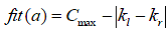
(8)

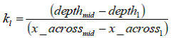
(9)

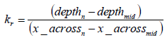
(10)

Where :

depth_i is the depth of beam i ;

x _ across_i is the across-track distance of beam i ;

k_l, k_r are the slope of the left measured depths respectively from the mid-point P_mid; C_max is a constant;

When the degree of deformation decreases, the value of fitness function fit (a) becomes larger while the becomes smaller. The actual observed measurements, provide more rigor and are retained when determining the solution.

4.2 Process of SVP Inversion

Figure 4 shows the SVP inversion process by GA.

First, the echo times (travel-times) of the terrain distortion are collected while the mode vectors and reconstruct coefficients ranges of the profiles are obtained by EOF in the survey area. Second, the SVP is reconstructed based on the above two elements and is used for the ray traced solutions for the bathymetry. By evolving with GA, the best individual measurements are preserved. Finally, the best reconstitution coefficient of the SVP is computed and the inversion result of the SVP is obtained.

5. Experiments

5.1 Inversion of the Sound Velocity Profile (SVP)

In this experiment, 11 SVP measurements were taken over 3 days are selected in during the survey area (Figure 5).period. The data of 70 pings arewere selected. One of the 11 measured SVPs is selected and inverted by the others. The process is measured SVPs and the EOF modeling results are shown in Figures 6 and 75 and Table 1 shows the 6. The computed ranges of the reconstruct coefficients are shown in Table 1.

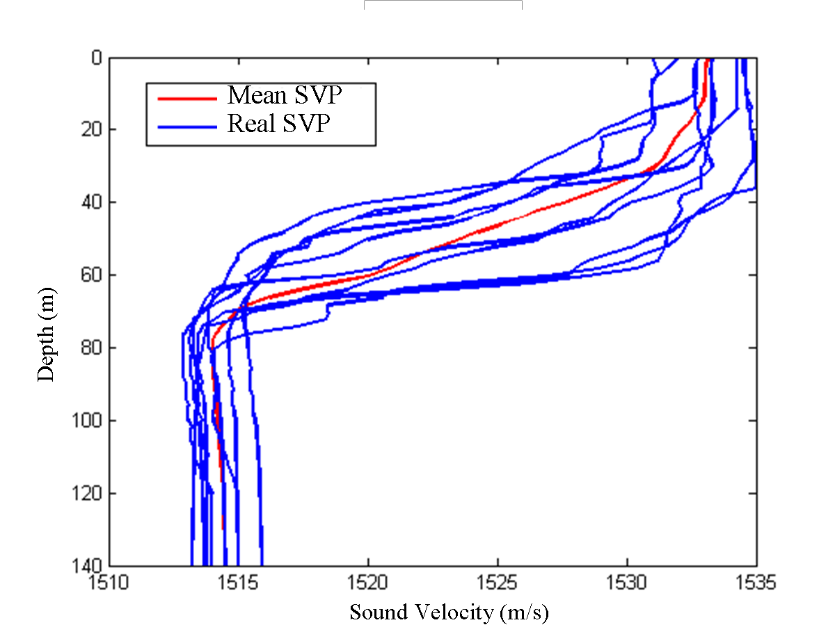
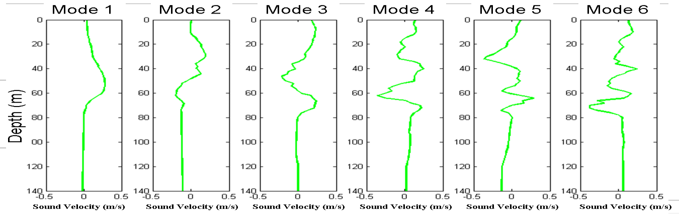
Based on the vectors and the 22nd ping of the bathymetry measurement, the SVP can be obtained by the method described in Section 4 (The energy of the SVP represented by the first six-dimensional vectors can reach above 96%).(HE, et al. 2011, ZHANG, et al. 2010).

According to the coefficient ranges in Table 1, the population can be initialized. The parameters for the GA method are:

Population Size: 50, Hybrid Probability: 0.8, Mutation Probability: 0.15, Cmax 100

After an evolution process of 2000 iterations, the optimal reconstruct coefficients are computed and listed in Table 2.

In Figure 7, the real, measured SVP is shown as a black line whereas the inversion result for the SVP is shown by the red line. The blue line shows the SVP which is nearest to the real SVP in time.

Comparing the error statistics (listed in Table 3) and the graphical results (Figure 7), it appears that the SVP obtained by inversion (red line), more closely estimates the real SVP (black line).

In Figure 8, the black line shows the actual seabed topography and this corresponds closely with the red line that shows the seabed topography derived from the inversion result of the SVP. The blue line shows the seabed topography which is nearest to the real SVP in time.

Statistical results shown in Table 4, indicates centimeter-level errors in the bathymetry based on the inversion SVP modeling.

5.2 Correction of Terrain Distortion by the Inversion SVP

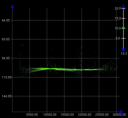
In Figure 9, the inversion SVP is used forleft hand image shows the ray traced solutions of two adjacent swaths:

6. Conclusions

In this paper, the influence of sound velocity error in determining seabed terrain is analyzed. According to the degree of the terrain distortion, a method for inverting the sound velocity profile (SVP) is proposed by combining EOF and GA methods. The design of a fitness function based on the terrain distortion provides the contents of the kernel to be used in the inversion process. The test results demonstrate that the terrain distortion caused by sound velocity errors can be effectively corrected by the SVP inversion results. Meanwhile, the accuracy of the multibeam bathymetry data has been significantly improved.

7. References

1. Cartwright, D.S,. (2003, Multibeam). Multi-beam Bathymetric Surveys in the Fraser River Delta, Managing Severe Acoustic Refraction Issues. M.Eng Report, University of New Brunswick, Canada.

2. DING Jisheng, ZHOU Xinghua, TANG Qiuhua, CHEN Yilan,. (2007,). Expression of MultibeamMulti-beam Echo Sounding Sound Velocity Profile with Empirical Orthogonal Functions, Geomatics and Information Science of Wuhan University 32(5): 446-449.

3. DONG Qingliang, CUI Minxun, ZHOU Junhua, WANG Jiguo, XU Yan. (2011). Analysis and Processing of Transform Geography of Convex and Concave in Multi-beam Sounding System, Hydrographic Surveying and Charting 31(1): 32-35.

4. DONG Qingliang, HAN Hongqi, FANG Zhaobao. (2007). The Influence of Sound Speed Profiles Correction on Multi-beam Survey, Hydrographic Surveying and Charting (2): 56-58.

5. HE Li, LI Zhenglin, PENG Zhaohui, WU LiXin, LIU JianJun. (2011). Inversion for sound speed profiles in the northern of South China Sea, SCIENTIA SINICA Phys, Mech & Astron 41(1): 49-57.

6. Herman, A.W, B. Beanlands, Chin-Yee M, Furlong A, Snow J, Young S, Phillips T. (1998). The Moving Vessel Profiler (MVP): in-situ Sampling of Plankton and Physical Parameters at 12 kts and integration of a new laser/optical plankton counter. Oceanology 98, 102: 123-135.

7. JIN G, Lynch J.F, CHIU C.S, Miller J.H,. (1996,). A theoretical and simulation study of acoustic normal mode coupling effects due to the Barents Sea polar front, with applications to acoustic tomography and matched field processing, J. Acoust. Soc. Am. 101(1): 193-205.

8. Kammerer E. (2000). New Method for the Removal of Refraction Artifacts in Multi-beam Echosounder Systems. PhD thesis, University of New Brunswick, Canada.

9. LeBlanc L.R & Middleton F.H. (1980). An underwater acoustic sound velocity data model, J Acoust Soc Am 67: 2055-2062.

10. LI Jiabiao, et al. (1999). Principles of multi-beam survey techniques and methods, Ocean Press, Beijing.

11. LI Jiabiao, Zheng Yulong, Wang Xiaobo. (2001). The Main Affecting Factors of Multi-beam Bathymetry Accuracy, Hydrographic Surveying and Charting (1): 26-32.

12. Lindsay C.E & Chapman N.R,. (1993,). Matched field inversion study of geoacoustic model parameter using adaptive simulated annealing, IEEE Journal of Oceanic Engineering 18(3): 224-231.

13. MATLAB Genetic Algorithm Toolbox and Application. (2005). XiAn University of Electronic Science and Technology Press, XiAn.

14. PENG LH, WANG L, QIU XF, TIAN J. (2003). Modal wave number tomography for South China Sea front, China Ocean Engineering 17(2): 289-294.

15. SHEN Yuanhai, MA Yuanliang, TU Qingping, et al. (1999). Feasibility of description of the sound speed profile in shallow water via empirical orthogonal function (EOF), Applied Acoustics 18 (2): 21-25.

16. Vaccaro R.J,. (1998,). The past, present and future of underwater acoustic signal processing, IEEE Signal Processing Magazine 7: 21-51.

17. ZHANG Xu, ZHANG Yonggang, ZHANG Jianxu, DONG Nan. (2011). A new model for calculating sound speed profile structure, ACTA OCEANOLOGI- CA SINICA 33(5): 54-60.

18. ZHANG Xu, ZHANG Yonggang , ZHANG Jianxue, NIE Bangsheng, YAO Zhongshan. (2010). EOF Analysis of Sound Speed Profile in East Water of Taiwan, Advances in Marine Science 28(4): 498-506.

19. ZHANG Zhongbing, MA Yuanliang, NI Jinping, et al, . (2002,). A New and Practical Method for Inverting Sound Speed Profile in Shallow Water, Journal of Northwestern Polytechnical University 20(1): 36-39.

20. ZHAO Jianhu, LIU Jingnan. (2009).

Multi-beam Bathymetric Survey and Image Processing, Wuhan University Press, Wuhan.

21. ZHU Xiaochen. (2011). Research on data processing critical modeling and application on multi-beam echo sounding. Dalian: Dalian Naval Academy, China.

7. Author Biographies

JIN Shaohua is currently a lecturer at the Department of Hydrography & Cartography of Dalian Naval Academy. He worked in the Naval Survey Troop from 2004 to 2005 and was appointed as the substitute captain of the survey unit. He has been lecturing since 2006 and was engaged in hydrographic surveying theory and data processing. He received his Doctor’s degree in Geodesy and Surveying Engineering in 2011. He has extensive experience in marine magnetic survey practice and data processing.

Email: jsh197835@163.com

SUN Wenchuan is currently a Ph.D. student in the Department of Hydrography & Cartography of the Dalian Naval Academy. He is engaged in hydrographic surveying theory and data processing. He obtained his Master’s degree in Geodesy and Surveying Engineering in 2012. He has extensive experience in marine magnetic survey practice and data processing.

Email: sunwch1986@163.com

BAO Jingyang is a Professor in the Department of Hydrography & Cartography of the Dalian Naval Academy. He worked in the Naval Survey Troop from 1987 to 1990 where he was appointed as the substitute captain of the survey unit. After receiving his Master’s degree from Dalian Naval Academy in 1995, he became a lecturer in the Department of Hydrography & Cartography in the same college. Following research and teaching in marine geodesy, he received his Doctor’s degree in Geodesy and Surveying Engineering in 2002 from Wuhan University. He was appointed Professor and supervisor of the Ph.D. program in 2005. He has extensive experience in tidal surveying practice and data processing.

Email: Jingyangbao@sina.com

LIU Min worked in the Naval Survey Troop from 2001 to 2005. He undertook postgraduate studies at Huazhong University of Science and Technology and received his Master’s degree in 2008. He is now a Ph.D. student of Information Engineering University, majoring in Geodesy. He has extensive experience in gravity theory and data processing.

CUI Yang is currently a lecturer in the Department of Hydrography & Cartography of the Dalian Naval Academy. She worked in the Naval Survey Troop from 2004 to 2005 and was appointed as the substitute captain of the survey unit. She has been lecturing since 2006 in marine geodesy, survey theory and data processing. She obtained her Doctor’s degree in Geodesy and Surveying Engineering in 2013. She has extensive experience in marine geodesy survey practice and data processing.

Email: 13998435151@163.com.