

Abstract
1 Introduction
In the hydrospatial domain (Hains et al., 2022), where accuracy underpins success, calibration and verification stand as the foundations of accurate and actionable data. Hydrospatial surveys provide critical insights into “all the blue of our blue planet and its contiguous zones” (Hains et al., 2022), the marine environments, facilitating marine exploration, environmental assessment, and subsea infrastructure development. Achieving these objectives depends heavily on the meticulous calibration and verification of advanced technologies such as Global Navigation Satellite Systems (GNSS) including Inertial Measurement Units (IMU), Multi-Beam Echo Sounders (MBES), and underwater positioning systems (LBL and USBL) and other related sensors deployed in the surveys. These sophisticated systems, commonly complemented by tools like Side-Scan Sonar (SSS), Magnetometers (MAG), Sub-Bottom Profilers (SBP), and Ultra-High Resolution Seismic (UHRS), demand rigorous calibration to minimize systematic errors and maintain data integrity (Lekkerkerk, 2024). Precision in Hydrospatial data is not just an aspiration; it is a professional mandate for Hydrospatial and even more specifically for certified hydrographic surveyors Level 0, 1 and 2, ensuring compliance with standards such as the International Hydrographic Organization (IHO) S-44 or project specific industrial standards. Calibration and verification are indispensable for reducing systematic errors, ensuring system integrity, and meeting industry standards such as IHO S-44 (IHO, 2020).
For hydrographic professionals, calibration and verification practices are more than procedural necessities they are an essential discipline. They validate system performance under real-world conditions, safeguard data reliability, and align outputs with contractual benchmarks and industry standards. The results enable informed decision-making, whether mapping complex seabed topographies, monitoring environmental changes, or planning subsea infrastructure in the Hydrospatial domain. Today in many modern hydrospatial surveys, the mobilisation of the vessel will be completed and signed off by the respective clients only after completion of successful calibration and verifications of the survey systems that are ready to be deployed. Hence this also mandate the calibration and verification for the survey industry.
Calibration and verification processes are crucial for achieving:
- Data accuracy and uncertainty: Calibration minimizes systematic errors and aligns sensors for optimal performance (IHO, 2020).
- System integrity: Verification confirms that systems operate as expected under real-world conditions.
- Standards compliance: Adherence to established industry standards, along with relevant national and international regulations, enhances the credibility and acceptance of survey results.
- Operational efficiency: Early identification and resolution of issues prevent expensive re-surveys and delays (Lekkerkerk & Theijs, 2013).
- Seamless integration: Ensures compatibility and alignment among GNSS, IMU, MBES, USBL, and other systems for comprehensive data acquisition (Schnare, 2014).
This article draws from the authors’ extensive experience in calibration projects, integrating standards and materials from IHO publications including Manual of Hydrography, Category ‘A’ and ‘B’ Hydrographic courses (S-5A and S-5B; IHO, 2018), and real-world surveying operations. It provides a concise overview of the importance of calibration and verification, equipping surveyors, especially junior professionals, with a robust framework to approach these critical processes.
The practices and principles outlined here are not exhaustive but are carefully organised to underscore the key technical depth and best practices that underpin successful all types of hydrospatial surveys. Having understand that there are many approaches for calibration and verification for the survey systems this guide reflects the dynamic interplay between theoretical knowledge and practical application, with an emphasis on fostering precision and reliability. As we navigate the complexities of marine surveying, this preamble sets the stage for a comprehensive exploration of calibration and verification methodologies, offering professionals a structured approach to mastering the tools and techniques that define excellence in the field.
Scope and contribution: This article focuses on the verification and calibration for positioning, attitude swath bathymetry and USBL as used in hydrospatial surveys. It does not attempt to reproduce all general practice material already documented in the IHO Manual on Hydrography (C-13; IHO, 2005); instead, it consolidates offshore procedures and error-control techniques and then links each step to the relevant C-13 clauses where applicable.
2 Positioning systems: verification and geodetic integrity
2.1 GNSS position verification in geophysical surveys: techniques and best practices
GNSS form the backbone of positioning in any hydrospatial including geophysical surveys, ensuring both horizontal and often also vertical accuracy for data acquisition (IHO, 2005). Accurate dimensional control and comparison of GNSS systems is critical to aligning survey systems with geodetic references and ensuring positional integrity across various survey operations. Although you cannot really calibrate a GNSS; this chapter explores the techniques, methodologies, and challenges associated with GNSS position verification, emphasizing its role in calibration and integration with other survey systems such as MBES and USBL. GNSS systems ensure that positional data is accurate and reliable, forming the basis for spatially consistent datasets. Verification of GNSS systems includes:
- Validating real-time positioning accuracy against reference standards.
- Ensuring offsets and lever arms are correctly accounted for.
- Cross-verifying primary and secondary systems using independent methods such as Real-Time Kinematic (RTK), Precise Point Positioning (PPP), or Post-Processed Kinematic (PPK).
- Validating final product positioning accuracies to meet the specific standards.
Primary and secondary GNSS systems. Position validation begins with a comparison between primary and secondary GNSS systems if available. These systems, typically integrated into the survey setup, operate using RTK or PPP corrections. The comparison ensures spatial consistency and accuracy in positioning, providing redundancy in case of primary system failures. The positions should be checked against project coordinates through the survey software to include any geodetic settings made in the survey software. Lever arms must be entered into the survey software with precision, as errors in these parameters can propagate through the system, affecting positional accuracy (IHO, 2005, Appendix 1 Part I).
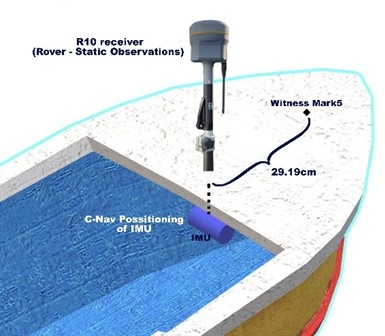
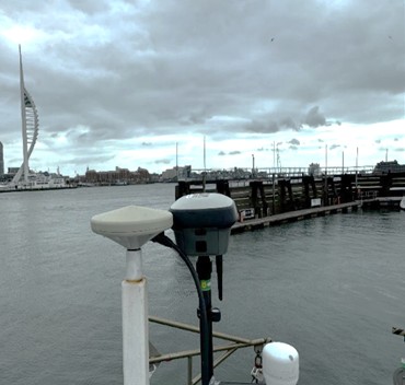
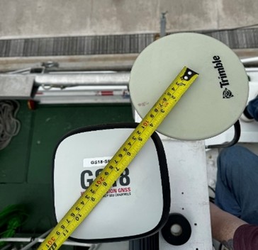
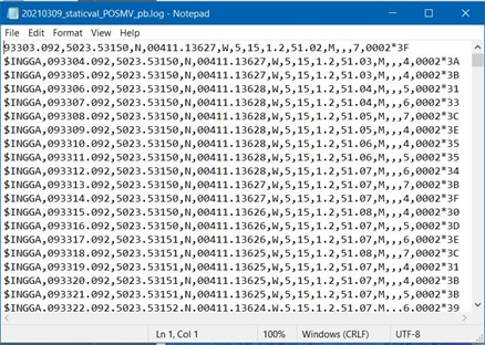
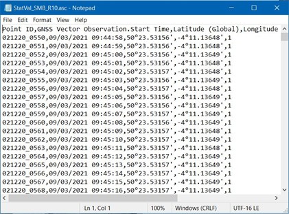
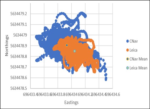
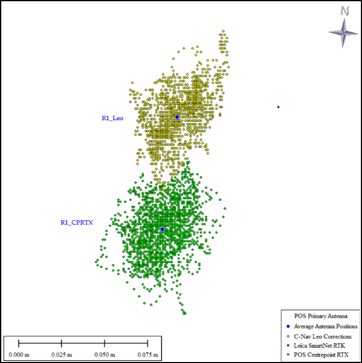
Independent verification using standalone GNSS systems. Standalone RTK GNSS systems or total station checks, provide an independent layer of validation. These systems offer precise positioning unaffected by biases in the primary setup, serve as an additional verification method, particularly in challenging environments or where the primary GNSS system’s data quality is questioned. On smaller vessels an (extra) antenna can also be placed directly over a benchmark to check the position output against the benchmark coordinates. Standalone GNSS systems or total station checks are often employed to validate positional accuracy independently. Setting up RTK receivers illustrate in Figs. 1 and 2. Further, different way of raw data and processed data representations can be found in Figs. 3 and 4.

2.2 Key considerations in positioning verification: limitations of numerical averaging
Numerical averaging, while a simple method for position determination, is not recommended for high-precision applications such as geophysical surveys.
Oversimplification: Numerical averaging of horizontal coordinates (X, Y) ignores the full 3D error ellipsoid inherent in GNSS data. This can lead to biased results, especially in cases where vertical uncertainty (Z) or correlated errors between axes are significant.
Error distribution: GNSS errors are not evenly distributed; atmospheric effects, satellite geometry, and multipath can introduce systematic biases.
Loss of covariance information: Numerical averages do not account for covariance between positional components, which is critical for understanding true positional uncertainty.
Hence the referred methods for positioning calculations are GNSS processing software, dedicated GNSS processing software offers advanced tools for deriving accurate positions:
- Weighted averaging: Observations are weighted by their estimated accuracy, ensuring that higher-quality data contributes more significantly to the final position.
- Error ellipsoid consideration: The software incorporates the 3D error ellipsoid, capturing positional uncertainties comprehensively.
- Residual analysis: By evaluating the residuals (differences between observed and modelled positions), the software identifies and excludes outliers, enhancing data reliability.
- Time-based integration: Longer observation times reduce the impact of random noise, a method particularly effective in static surveys.
These capabilities make GNSS processing software indispensable for high-precision applications, such as control point establishment and baseline verification.
2.3 Absolute position validation
Validate lever arms by comparing GNSS-derived positions with those calculated from IMU measurements during static and dynamic tests. This could be done by using a separate (RTK) GNSS unit placed on corners of the vessel and comparing the obtained coordinates with those produced from the vessel main GNSS through the ship reference frame (SRF) and IMU / gyro towards the node on which the separate GNSS is placed. By placing the separate GNSS on the extremities any errors in alignment can be noted. Document this as a pre-survey verification in line with C-13 checklists (IHO, 2005, Appendix 1 Part I).
3 Motion reference systems: alignment, calibration, and performance
3.1 Gyro / heading sensor alignment against the SRF
Accurate heading data is indispensable in hydrographic surveys, ensuring precise alignment of positioning and survey lines with real-world coordinates. Errors in gyro compass readings can result in inaccuracies in bathymetric geophysical data and any hydrospatial data, making calibration a critical component of survey preparations (Royal Navy, 2019). A gyro compass with a recent manufacturer calibration report serves as the baseline for surveys (calibrated gyro). However, verifying the alignment of the gyro with the SRF is essential.
Modern surveys increasingly rely on GNSS-aided heading systems and Fibre Optic or Ring Laser gyros. Integrating an aligned gyro compass with other survey systems, such as MBES and USBL, ensures heading discrepancies remain within acceptable. This integration is essential for maintaining alignment between survey lines and geodetic coordinates. Verifying the alignment of heading systems and cross-referencing with transits or established heading references such as light lines or sun azimuth checks enhances the overall reliability of the survey data. Such practices not only meet industry standards but also build redundancy and resilience into the survey workflow, ensuring high data integrity in hydrographic operations.
Heading alignment ensures the correct alignment of the vessel or survey platform. It is used to determine any alignment errors between the gyro and the SRF.
Methodology: Two positions along the centreline of the vessel (bow-stern SRF axis) at known, fixed locations on the vessel or platform. These positions can be determined using two GNSS receivers but also using a total station or through (tape) measurements from a reference heading such as a quay of which the heading was determined using a topographic survey. The true heading of the vessel is computed and at the same time the output from the gyro is observed. The difference between the two gives the computed-observed (C – O) correction. Care should be taken when grid headings are compared with calculated values, incorporating projection corrections to account for grid convergence. Fig. 5 illustrate schematic of vessel reference frame and GNSS aided heading. For combined gyro-IMU instruments, the gyro C – O must be implemented in the instrument (not only in the acquisition software) before IMU alignment, to eliminate roll- pitch cross talk at the source. Grid convergence (γ) is the angle between the projection or chart north and true north. It varies across the projection, depending on the point’s position relative to the origin of the projection. In a UTM projection the origin is the central meridian of the UTM zone but in other projections this may be a central point or parallel. Fig. 6 indicate the relation of grid north and true north. Grid convergence conventions vary from projection to projection and may also differ depending on the formula used.
Software tools like CARIS, QGIS, or Trimble GNSS software can compute grid convergence automatically. However, it should always be ensured that the C-O correction of the gyro compass is entered as a true north correction, free of any convergence.


3.2 Inertial measurement unit and gyro against SRF
This alignment must be performed only after the gyro/heading alignment has been completed and the gyro C – O applied in the instrument for integrated units. In the context of hydrospatial surveys, the Inertial Measurement Unit (IMU) plays a pivotal role in ensuring accurate motion compensation by measuring accelerations and angular velocities. This is especially critical in marine environments, where vessel dynamics introduce complex motion patterns. Proper alignment of the IMU against the SRF ensures seamless integration with other systems, such as GNSS and MBES, and enhances the overall quality of survey data. This chapter provides a comprehensive guide to the alignment of IMU systems on board survey vessels, focusing on industry best practices, methods, and tools for precise alignment and validation (IHO, 2005, Chapter 7).
The IMU measures the vessel’s motion in six degrees of freedom: three linear accelerations (surge, sway, and heave) and three angular rotations (roll, pitch, and yaw). Aligning the IMU (often erroneously called calibration) ensures that the IMU data aligns with the SRF. Lever arms and offsets between the IMU, GNSS antennas, and other on-board sensors are accurately accounted for and Integration errors are minimized. There are mainly two types of ‘calibration’ for IMU system: factory Calibration and Onboard alignment. Factory calibration is performed by the manufacturer and focuses on ensuring that the IMU output is correct with regard to the internal reference frame of the sensor itself. This includes:
- Sensor biases: Correcting systematic measurement errors.
- Scale factors: Adjusting the sensitivity of each sensor.
- Alignment: Aligning IMU sensors with its internal reference frame.
Factory calibration ensures the IMU operates within specified tolerances under ideal conditions but does not account for vessel-specific installation factors. Periodic factory calibrations are recommended per manufacturer’s standards and needs. Alignment focuses on aligning the IMU with the vessel’s coordinate system (SRF). This includes:
- Accounting for lever arms (offsets between the IMU, GNSS antennas, and other sensors).
- Correcting installation angular misalignments.
- Validating dynamic performance under survey conditions.
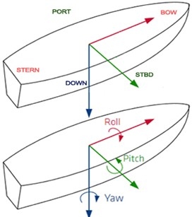
Dimensional Control (DIMCON) survey is a fundamental procedure in hydrographic surveying, ensuring precise spatial measurements of offsets between key survey equipment components. This process involves advanced accurate land survey techniques, such as the use of total stations, laser scanners or photogrammetry, to determine the lever arms and spatial relationships between GNSS antennas, MBES systems, USBL transducers, and IMUs within the SRF. Regular updates to DIMCON surveys are essential, especially after any equipment modifications or changes to sensor mountings and locations, as these trigger the need for redetermination. While there is no specific validation period for DIMCON, ongoing node verifications can provide valuable insights into any potential changes in DIMCON values. However, it is considered good practice to conduct a DIMCON survey roughly every few years, even if no modifications have been made, as advancements in methodologies and survey accuracies may result in updated and more precise offset measurements. This procedure not only mitigates alignment errors but also optimizes data reliability for both dynamic and static survey operations. It is very important to understand different conventions for the offset by different manufacturers. Fig. 7 illustrates the different approach by few industrial standard software and system for the offset and rotation conventions.
The optimal IMU on a survey vessel is not solely determined by its proximity to the vessel’s centre of gravity (COG) but rather by a strategic balance between minimizing lever arms and reducing motion-induced errors. While manufacturers often recommend installing the IMU near the COG, a more precise approach considers the vessel’s pivoting centre to minimize accelerations and mitigate ‘false heave’ effects. In modern survey configurations utilizing RTK or PPP corrections for height, false heave is significantly reduced, making rotational accuracy a more critical factor. Consequently, a few installation strategies exist: one prioritizes the reduction of lever arms to minimize rotational errors, while the other places the IMU at the vessel’s centre of rotation to limit accelerations. For “all-on-the-pole” setups, an optimal position is near the waterline, between the GNSS and MBES, ensuring better alignment and data consistency. Given these considerations, the best placement is survey-specific, requiring an evaluation of vessel dynamics, system integration, and operational requirements (Lekkerkerk & Theijs, 2013) When initially installing the IMU onboard ensure the mounting is rigid to prevent relative movement between the IMU and the vessel. Then enter approximate lever arms into the system software based on DIMCON survey results. Align the IMU with the vessel’s reference frame (fore-aft, athwart ship, and vertical axes). Ensure that the unit is aligned with the SRF in all three dimensions to prevent ‘cross-talk’, i.e. for example a pitch motion inducing a false roll motion due to a yaw offset of the IMU. Perform Lever arm calibration which determines the offsets between the IMU, GNSS antennas, and other reference points.
Alignment calibration addresses misalignments between the IMU’s internal axes and the vessel’s reference frame. Vertical axis misalignments of the MRU are particularly problematic, as they introduce crosstalk between pitch and roll angles. This is especially critical for outer beams of wide swaths (e.g., 120°), where even a minor yaw misalignment (e.g., 2°) can result in seabed “wobble” errors of up to ±10 cm in 20 m water depths. This wobble, primarily roll induced by pitch, is difficult to eliminate due to the challenge of aligning the MRU with the SRF at its mounting location (de Hilster, 2009). Nicolàs de Hilster explain in his article series on Hydro International (The MRU and SRF Aligned) the principles of the Dutch method for MRU alignment, developed by the Survey Department of Rijkswaterstaat (the Directorate-General for Public Works and Water Management of the Netherlands). The method addresses both vertical axis alignment with the SRF and the correction of pitch and roll angles. For this article, only the vertical axis alignment is considered (de Hilster, 2009); readers are referred to the articles for a detailed explanation.
Some GNSS aided IMUs, and INS (such as POSMV systems) require an alignment against the SRF followed by an alignment between the GNSS antenna’s and the IMU (heading alignment). As this is difficult to do under stationary conditions this is done using a dynamic alignment. Dynamic alignment involves executing specific manoeuvres and leveraging GNSS data to detect and correct misalignments in pitch, roll, and yaw, as well as synchronizing data streams to eliminate latency discrepancies. Straight-line runs at constant speeds identify fore-aft misalignments, while controlled turns assess heading (yaw) and athwartship (roll) errors by comparing angular velocity data from the IMU with GNSS-derived headings. GAMS (GNSS Azimuth Measurement Subsystem) calibration further refines the alignment of GNSS antennas, reinforcing and validating DIMCON results for optimal IMU performance in geophysical surveys. In integrated units, perform gyro alignment first, apply the gyro C – O in the instrument, and then carry out dynamic alignment and subsequent checks.
Analyse roll, pitch, and yaw data for unexpected variations or noise.
Best practices for onboard IMU calibration:
- Verify all hardware and software are functioning correctly.
- Verify sign conventions in both unit and software
- Conduct a DIMCON survey before mobilization to measure lever arms.
- Align regularly: Perform alignment at the start of every project or when equipment configurations change.
- Document results: Maintain detailed records of calibration parameters and verification results.
- Include reports generated by software aids.
- Train survey teams: Ensure team members are familiar with calibration procedures and equipment.
- Produce a short alignment verification note and attach plots to the pre-survey file, following the structure suggested in C-13 Appendix 1 (IHO, 2005).
IMU alignment is an essential process in marine surveys, ensuring accurate motion compensation and seamless integration with GNSS and MBES systems. By adhering to structured calibration procedures and leveraging advanced tools, surveyors can minimize errors, enhance data quality, and meet industry standards. Regular calibration and verification not only ensure compliance but also build confidence in the reliability of survey data, making it indispensable for professional hydrographic operations.
3.3 Integrated INS (Gyro_IMU) alignment workflow and GAMS
For the modern integrated units (gyro + IMU/INS), perform gyro/ heading alignment first and apply the gyro C – O in the instrument to suppress roll – pitch cross talk before any IMU alignment. Then execute an INS dynamic alignment (straight runs and controlled turns) to solve installation angles and confirm timing, followed by GAMS/dual antenna heading calibrations, which is technically a separate GNSS azimuth subsystem integrated to refine heading and validate DIMCON.
4 Swath Systems: Calibration and Quality Assurance
4.1 Alignment and verification of MBES systems
Sound Velocity Profile (SVP) verification is a critical step in ensuring the accuracy of survey data, particularly for systems reliant on sound velocity for calculations, such as MBES), USBL positioning systems, and data acquisition platforms like QINSy and SIS. Using tools like the SVP or Moving Vessel Profiler (MVP), surveyors can capture updated and precise sound velocity data at varying depths to mitigate refraction errors and ensure accurate beam steering. Regularly updated SVP data is essential for calibrations, as deviations in sound velocity can introduce significant errors in depth, positioning, and acoustic data processing. By integrating real-time or recently measured SVP data into survey operations, professionals ensure optimal system performance and adherence to industry standards such as IHO S-44. Most modern MBES systems require not only a separate SVP, MVP or CTD to measure the sound velocity profile but also require a separate sound velocity measurement near the transducer to properly compute the direction of the receives acoustic information. The values from this sensor should be cross referenced to those from comparable depths using the SVP / MVP or CTD.
Alignment is a critical step in ensuring the accuracy and reliability of MBES systems, particularly for dual-head setups. These systems, widely used in Hydrospatial surveys, require precise adjustments to account for offsets in pitch, roll and yaw. Accurate alignment determines the transducers axes with the SRF, reduces systematic errors, and enhances data integrity, enabling compliance with standards like the IHO S-44 for safety of navigation. This chapter delves into the essential calibration processes, with a focus on dual-head systems, while emphasizing best practices and practical considerations for effective alignment and verification.
For the purposes of estimating the resultant beam vector (the intersection of transmit and received steered cones) in the local level coordinate systems, the patch test is adequate as it solves for the sonar to SRF misalignments as well as the latency (or lack thereof when precise time stamping is used) between the GNSS and MBES. But without a proper alignment of either (and thus by inference both as they are only relatively aligned) sensor with respect to the SRF, the lever arm offsets cannot be applied correctly (Clarke, 2003).
4.2 Patch test calibration
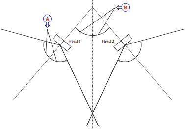
The patch test is designed to address angular offsets in the MBES system. For dual-head MBES setups as illustrated in Fig. 8, each transducer head must be calibrated independently to ensure cohesive data output. The calibration process includes adjustments for pitch, roll, yaw, and latency, conducted through carefully planned survey lines.
4.3 General conditions for patch testing
- Conduct tests in calm weather and low current conditions to minimize noise and motion artifacts.
- Use a flat seabed at a depth at least equal or deeper to those encountered in surveying or distinct sloping terrain (preferably slope between 1:2 and 1:5), depending on the specific calibration parameter.
- Maintain steady vessel speeds, with variations for latency calibration. Perform all previously described tests, alignments and verifications.
- Obtain a recent sound velocity profile and enter it into the software;
- Ensure sufficient overlap of beams for both heads during calibration.
Most software packages have automated routines for the patch test. While there is nothing against these routines the prudent surveyor should always visually check the results by applying the suggested values and inspecting the resulting bottom for any remaining discrepancies.
4.4 Roll calibration
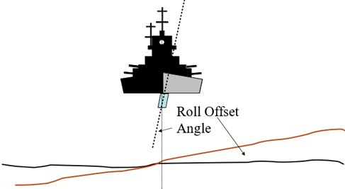
Roll calibration addresses angular misalignment along the vessel’s port-starboard axis; roll offset illustrate in Fig. 9, typically the most sensitive offset to correct.
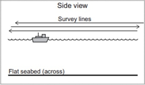
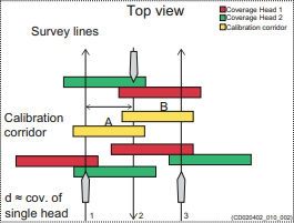
Line Plan: For a single head, sail the same (theoretical) line in opposite direction over a flat bottom. For dual head, use three parallel lines over a flat seabed one central and two with lateral offsets. Ensure these lines provide overlapping beams from each transducer head.
Procedure: Analyze the outer beams from overlapping data to isolate roll offsets. A flat seabed ensures that observed discrepancies are due solely to roll misalignment.
Dual-Head consideration Fig. 10: Treat port and starboard heads individually. Roll errors in one head may not align with those in the other, necessitating separate corrections.
Record conditions, line plans, and results as part of the C-13 Appendix 1 pre-survey / survey records, including Annex E SVP entries (IHO, 2005).
4.5 Pitch calibration
Pitch calibration corrects fore-aft angular misalignment of the transducers relative to the vessel’s longitudinal axis.
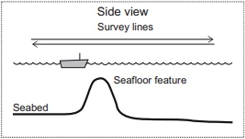
Line Plan: Run two lines as indicated in Fig. 11, over a sloping seabed in opposite directions (uphill and downhill). Ensure overlapping coverage for port and starboard heads. Avoid lateral offsets in the lines to maintain data consistency.
Procedure: Compare the profiles from the two lines. Any pitch error will visible as a growing discrepancy in depth as distance increases.
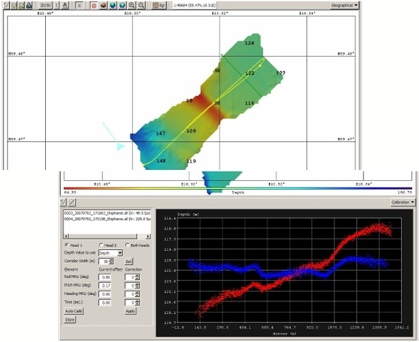
Dual-Head Consideration: Each head must be treated as a separate entity. Overlap data from individual transducers to isolate pitch offsets effectively. Fig. 12 illustrate Patch test interface of Caris HIPS & SIPS processing software. Survey line plan recommendation for pitch calibration illustrate in Fig. 13.
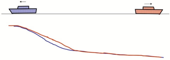
Fig. 11 Line plan for pitch calibration (SIS, 2024).
4.6 Yaw (heading) calibration
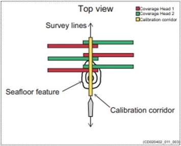
Yaw calibration corrects rotational misalignment between the transducers and the vessel’s heading. Line Plan: Single head: run two lines across a distinct target or slope with the two lines overlapping each other. Dual head illustrate in Fig. 14: Run three lines across a distinct target (e.g., a wreck) or slope with the second line crossing the target at 90 degrees.
Ensure lateral spacing of 1.5x the water depth between lines for optimal sensitivity. Heading calibration of a dual head system will need careful planning. Run 3 lines as indicated below with the 2nd Line crossing a distinct object STB Head: Select line 1 and 2, make a calibration corridor along the centre beam of line 2.
PORT Head: Select line 2 and 3, make a calibration corridor along the center beam of line 2.
Procedure: Compare the central beams from overlapping data. Any heading misalignment will cause the target positions to deviate. Adjust offsets in the software to align targets. Dual-Head Consideration Fig. 15: Perform separate yaw calibration for each head. For the starboard head, use lines 1 and 2; for the port head, use lines 2 and 3. Create calibration corridors along the central beams for precise analysis.


4.7 Latency calibration
Latency calibration ensures synchronization between positional data and acoustic measurements. Yaw calibration is performed using crossing lines over distinct features, while latency calibration overlays lines at varying speeds to detect timing discrepancies (Lekkerkerk & Theijs, 2019).
Line Plan: Run two lines over a distinct feature at distinctly different speeds as illustrated in Fig. 16 (e.g., 3.5 knots and 7 knots).
Procedure: Overlay the data from the two lines. Any latency offset will cause positional discrepancies, which can be corrected in the system settings.
Best Practice: Use PPS (Pulse Per Second) timing where available, as it minimizes latency issues.
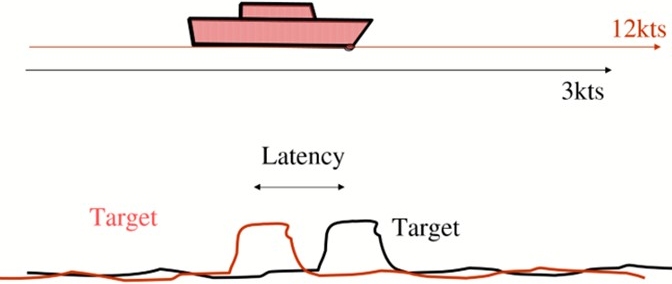
Fig. 16 Survey lines for patch test: Latency calibration (SIS, 2024).
4.8 Post-calibration verification
Verification ensures that the calibration process has effectively addressed all offsets and that the MBES system meets required accuracy standards. This involves repeatability tests, noise analysis, and cross-track error assessments. Reputability is surveying a known feature (e.g., a wreck or underwater structure) in opposite directions. Compare overlapping data for depth consistency and accuracy.
MBES Integration; Use MBES data to verify motion compensation accuracy by analysing beam footprints and depth consistency. For example, roll the vessel in a heavy sea and check if a flat bottom remains flat in the recorded data.
Cross-Track Error Assessment: Validate positional accuracy using cross-track and along-track error metrics and confirm compliance with project-specific tolerances.
4.9 Best practices for dual-head systems
Efficient line pattern for dual head system recommended in Fig. 17. The alignment of MBES systems, particularly dual-head configurations, is a meticulous process that requires careful planning, execution, and verification. By addressing angular offsets through patch testing, surveyors can achieve high-precision bathymetric data.

4.10 Absolute depth check
After the calibration and verification of the MBES as outlined above a further check should be made to verify that the depths as measured are correct with regard to the chosen vertical datum. This can be accomplished by checking the obtained depths against an independent reference. This could be a topographically surveyed sill of a set of locks, a bottom with known depth or even against a lead and line (and tidal) measurement near the nadir of the MBES. Care should be taken that the depths taken independently are compared against the depths as processed in the proper vertical datum through the survey software to verify all alignments and settings in the software.
5 Underwater positioning and system calibration
5.1 Calibration of USBL systems: a technical guide
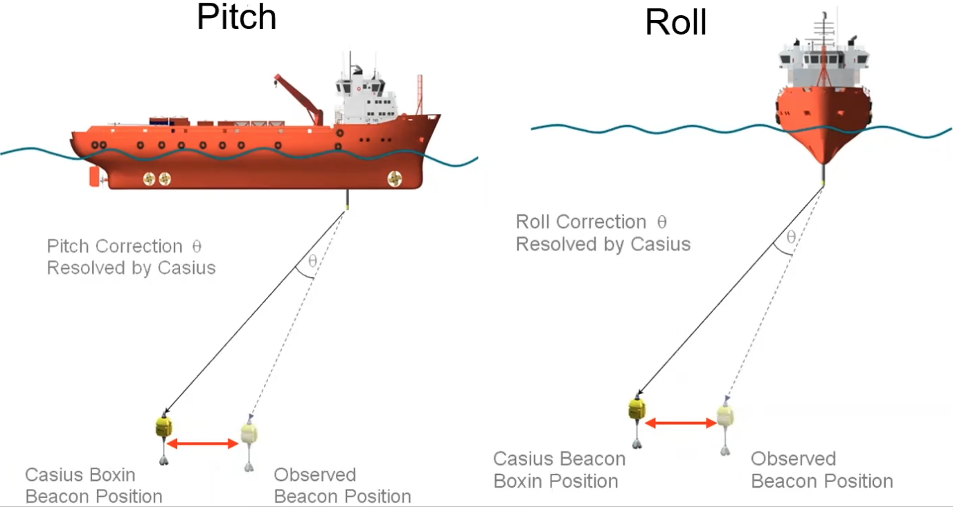
Ultra-Short Baseline (USBL) systems are pivotal in subsea positioning, particularly for the accurate deployment and tracking of remotely operated vehicles (ROVs), towed equipment, and underwater sensors. A USBL Calibration is essential to ensure correct electronic alignment of the vessel’s USBL acoustic, GNSS and attitude sensor offsets. This chapter outlines a professional and structured approach to USBL calibration, focusing on the widely preferred box-in calibration method, along with considerations for verification and best practices. Verification involves comparing observed beacon positions with theoretical coordinates, ensuring compliance with project-specific tolerances and industry benchmarks. Some USBL systems include a built-in motion reference unit. These systems are calibrated in the factory and the electronic offsets are known and set prior to delivery. These systems usually require no calibration, but a verification test is recommended upon installation to correct any physical heading, pitch and roll errors, and to check the GNSS offsets for absolute positions of USBL contacts.
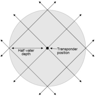
USBL Calibration: Box-In Method; Box-in calibration is the most commonly used method for USBL systems, ensuring precise alignment and correcting for latency. This approach uses predefined survey lines around a beacon to collect data for detailed analysis. While box-in calibration is preferred for its accuracy and flexibility, vessels equipped with dynamic positioning (DP) systems can opt for static calibration in certain scenarios. Fig. 18 shows the radius of the offset at ⅓ water depth; however, this is only for deep water (1000m+) calibrations where the DP vessels tend to operate.


5.2 Calibration procedure
Calibration procedure describes here specify for the shallow water USBL calibration approach as the context for the document is more focus on survey using MBES (usually shallow water operations). Hence, include only the techniques and associated diagrams for shallow water calibrations are used bellow.
offshore vessels using USBL for the purposes you described above will conduct USBL Calibrations at significantly greater depths. Arguably the optimum depth for a USBL Calibrations is over between 300 m and 1000 m. The technique you describe for the USBL calibrations will produce good results at these depths, but not so good at 35–50m depths due to refraction errors and thruster wash experienced at the high angles of attack for acoustic ranges.
Beacon Deployment: Position the beacon at a fixed and known depth, typically between 35–50 m (Depending on the project and general depth of the area or as per the manufacture guidelines for the specific system), ensuring that it is free from obstructions or significant underwater noise. Beacon can deploy in floating (3–5 m above the seabed with help of Float collar) or in a fix frame on the seabed. Document beacon deployment depth, mooring type, and environmental conditions in (IHO, 2005, C-13 Appendix 1, survey log).
For the shallow water depths (30–50 m) it is recommended that only a fixed frame is used, or a very short tether of less than 0.5 m. This is to reduce errors in the beacon position introducing errors into the vessel calibration result. A 3–5 m tether in 35–50 m of water will be subject to significant sway caused by current, and the beacon position may move by up to 3 m (up to 10 % of the water depth) during the calibration invalidating the results by introducing large systematic errors. In deep water the sway offset of a tethered is a far smaller percentage of the overall systematic errors (0.03 %), and therefore more acceptable. However, with some USBL systems delivering accuracies of 0.01 % of water depth, fixed frames are still best for a Box-in style calibration.
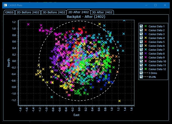
Remember you are calibrating against a fixed known refence. The pre-calibrated beacon position results for each run will see differences in the calculated result. (2D before plot). The CASIUS or QINSY software will then make/suggest changes to sensor offsets to align the position results into one point (2D after plot). The operator can QC the data, make informed changes to other settings such as sound speed, and error rejection filters to fine tune the results for the best calibration result. Sonardyne CASIUS (Calibration of Attitude Sensors in a USBL System) software, when run directly from Ranger 2 will apply the final changes to system and produce a calibration report. Operators using QINSY or other USBL systems apply the changes manually. The results can then be verified post calibration.
Survey Line Design (Deep water line pattern): Run 12 lines around the beacon: Four lines in cardinal directions: North (N), South (S), East (E), and West (W). Two diagonal crossings to enhance data density and improve angular accuracy.
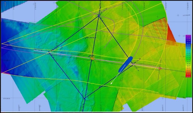
Data Processing: Process the acquired data using specialized software such as CASIUS, QINSy, or equivalent. Store before/after calibration plots and software reports with (IHO, 2005, C-13 Appendix 1, calibration record). The software computes alignment and latency corrections, ensuring the USBL system aligns seamlessly with the vessel’s reference frame. These are profiles sailed for deep water USBL calibration of 1000 m + water depths. It would be very challenging to sail this profile at ⅓ water depth with a beacon deployed at 30 m. Hence for shallow water survey the vessel sailing a four-leaf clover profile extending to 50 m from beacon position are recommended as illustrated in Figs. 19 and 20. Recommended deployment of USBL calibration procedures for shallow water shown in Fig. 21.
Example report of a CASIUS and data representation within the Ranger2 software interface illustrated in Fig. 22. While performing a real world USBL calibration, a screen capture for QINSy Navigation screen taken by author in Fig. 23.
Key considerations for box-in calibration:
- Lateral offsets: Maintain lateral offsets proportional to 33–50 % of the water depth (max. offset 500 m) for optimal coverage and accuracy.
- Vessel speed and stability: Ensure a steady course and maintain a survey speed of 3.5 knots throughout the calibration process.
- Environment: Select a calibration area with minimal underwater noise and interference to improve data clarity.
- Data Verification: Validate processed results against industry benchmarks to ensure alignment and latency corrections meet project requirements.


5.3 Verification of USBL systems
Purpose and Importance; Verification ensures that the USBL system’s calibration has been executed correctly and that its accuracy aligns with project-specific tolerances. Verification is critical to confirm that positional deviations are within acceptable limits.
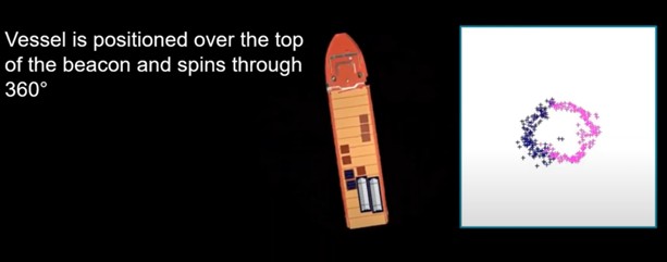
Spin Test: A spin test in Fig. 24 involves rotating the vessel around the deployed beacon at a steady rate. This evaluates the system’s pitch and roll offsets, and GNSS offsets for absolute positioning errors and its ability to maintain accurate positioning during rotational movements.
Walk-Away Test: Move the vessel away from the beacon at a steady speed Fig. 25, observing and recording positional data to confirm heading offset alignment and the calibration’s reliability over varying distances.
Ensure deviations fall within acceptable tolerances as outlined in project specifications or industry standards. Spin checks and walk-away tests further validate the calibration’s stability and accuracy under operational conditions.
Mobilisation remains one of the most demanding and critical phases of any hydrographic survey, regardless of its scope. While this article has focused on the GNSS, MBES, and USBL systems, it is important to recognise the broader array of sensors within the hydrospatial domain such as magnetometers, SSS, SBP, and SVP, including MVP and many other sensors. Each of these instruments requires specific calibration and verification procedures such as spanner tests and positional verifications for SSS, surrogate item tests (SIT) for MAG, and SVP comparisons to ensure optimal performance and many other test, calibrations and verifications for individual system. Completing these checks is essential for formally signing off the mobilisation phase and authorising the commencement of survey operations. As hydrographic surveyors, it is imperative not only to perform these procedures but to understand the theory behind them, ensuring confidence, reliability, and accuracy throughout the survey lifecycle.
6 Discussion: error propagation, verification value, and limits of guidance
Calibration reduces systematic components of error, while verification demonstrates fitness-for-purpose under operating conditions. Errors propagate through lever arms, timing, refraction, and heading alignment; their combined impact is most visible in outer-beam depth bias, seafloor “wobble,” and target positional spread. Offshore practice often extends beyond general guidance in C-13 (IHO, 2005), which treats such topics across positioning, depth, and practice chapters and in Annex E rather than in a single “calibration” chapter. The framework presented here therefore complements C-13 by linking everyday offshore procedures (patch tests, INS dynamic alignment, USBL box-ins) to S-44’s uncertainty outcomes and to traceable records in (IHO, 2005, Appendix 1), offering a practical bridge between standards and operations.
7 Conclusion
Calibration and verification are not supplementary tasks but the cornerstones of hydrospatial survey integrity. The technical frameworks described in this report covering GNSS verification, IMU alignment, gyro calibration, MBES patch testing, and USBL calibrations demonstrate that systematic validation directly safeguards data quality, reduces operational risk, and ensures compliance with international standards such as IHO S-44 for safety of navigation and other industrial standards. Mobilisation phases now routinely require formal calibration sign-off before survey commencement, underscoring their role as contractual and professional imperatives. By tying each procedure to C-13 record-keeping and S-44 uncertainty criteria, the workflow becomes both defendable and repeatable (IHO, 2005).
Beyond compliance, rigorous calibration fosters confidence in the results, enhances the interoperability of complex sensor suites, and prevents costly re-surveys or project delays. Importantly, these practices also serve as a training foundation for the next generation of hydrographic professionals, instilling precision, accountability, and a structured approach to system verification. As hydrospatial operations expand in scope and complexity driven by offshore energy, environmental stewardship, and subsea infrastructure the ability to execute reliable calibrations will remain a defining standard of excellence. Continuous peer collaboration, analysis of recurring calibration issues, and adherence to best practices will not only uphold operational quality but also contribute to the evolution of hydrospatial standards. Ultimately, calibration and verification are not just technical necessities, but professional disciplines that underpin the trust, safety, and credibility of hydrographic survey operations worldwide.
References
Clarke, J. (2003). A reassessment of vessel coordinate systems: what is it that we are really aligning? Proceedings of the US Hydrographic Conference. pp. 1–12. https://api.semanticscholar.org/CorpusID:111076905 (last accessed 1 November 2025).
de Hilster, N. (2009). The MRU and SRF Aligned. Hydro International. https://www.hydro-international.com/content/article/the-mru-and-srf-aligned-ii-and-iii (last accessed 1 November 2025).
DrillingFormulas (2016). Magnetic Declination and Grid Convergent and Their Applications in Directional Drilling. Drilling Formulas and Drilling Calculations, Grapevine, USA. https://www.drillingformulas.com/magnetic-declination-and-grid-convergent-and-their-applications-in-directional-drilling/ (last accessed 1 November 2025).
Hains, D., Schiller, L., Ponce, R., Bergmann, M., Cawthra, H. C., Cove, K., Echeverry, P., Gaunavou, L., Kim, S.-P., Lavagnino, A. C., Maschke, J., Mihailov, M. E., Obura, V., Oei, P., Pang, P. Y., Njanaseelan, G. P., Sharma, S. L. (2022). Hydrospatial – Update and progress in the definition of this term. The International Hydrographic Review, 28, pp. 221–225. https://doi.org/10.58440/ihr-28-n14
IHO (2005). Manual on Hydrography (1st ed.). IHO Publication C-13, International Hydrographic Organization, Monaco. https://iho.int/uploads/user/pubs/cb/c-13/english/C-13_Chapter_1_and_contents.pdf (last accessed 1 November 2025).
IHO (2018). Standards of Competence for Category ‘A’ Hydrographic Surveyors (ed. 1.0.2). IHO Publication S-5A, International Hydrographic Organization, Monaco. https://iho.int/iho_pubs/standard/S-5/S-5A_Ed1.0.2.pdf (last accessed 1 November 2025).
IHO (2020). Standards for Hydrographic Surveys (ed. 6.0). IHO Special Publication S-44, International Hydrographic Organization, Monaco.
Lekkerkerk, H.-J. and Theijs, M. J. (2013). Handbook of Offshore Surveying (Volume III). Skilltrade, London, UK.
Lekkerkerk, H.-J. and Theijs, M. J. (2019). Handbook of Offshore Surveying (Volume I). Skilltrade, London, UK.
Lekkerkerk, H.-J. (2024). S-44 and the systematic error. Hydro International. https://www.hydro-international.com/content/article/s-44-and-the-systematic-error (last accessed 1 November 2025).
Royal Navy (2019). The Admiralty manual of navigation: Vol. 1: Principles of navigation (11th ed.). The Nautical Institute. ISBN 9781906915643.
Schnare, T. (2014). Caris HIPS & SIPS 8.0 Manual for Hydrography & Survey Use. MGEO 2014.
SIS (2024). Seafloor Information System Reference Manual (ed. 5.12).K ongsberg Discovery AS, Norway.
Sonardyne (2020). Sonardyne Training Webinar 7 – CASIUS [Video]. YouTube. https://www.youtube.com/watch?v=yuIHhlinMh4 (last accessed 1 November 2025).