


Abstract
1. Introduction
National hydrographic offices are mandated to guarantee safe navigation across their marine territories through the production of quality nautical charts (Fisheries and Oceans Canada, 2017). Conventionally, the acoustic-based technologies, such as multibeam echosounder (MBES) systems, have been primarily relied on in nautical chart production. However, these conventional technologies have also displayed a critical limitation in extending bathymetric coverage towards nearshore shallow waters, where ship accessibility has been restricted due to ship draft and complexity in seafloor terrain (Scharff, 2007). This inaccessibility during a hydrographic survey has traditionally resulted in uncharted nearshore regions, also widely known as “white ribbon” gaps, persisting on nautical charts (Kotilainen & Kaskela, 2017). Uncharted extents on nautical charts raise a potential risk for the mariner to encounter ship accidents with shoals near these uncharted areas. To address this limitation, Airborne Light Detection And Ranging (LiDAR) Bathymetry (ALB) progressively emerges as a promising alternative to acoustic-based technologies in mapping coastal regions, considering the capability of ALB to fill in those “white ribbon” gaps. Still, the credibility and reliability of ALB in nautical chart production requires further validation for broad acceptance. It is, therefore, worth investigating the performance of ALB in shallow water bathymetry for navigational safety (Saylam, Hupp, Averett, Gutelius, & Gelhar, 2018).
In this paper, qualitative and quantitative systematic approaches that include adapting a widely accepted surface differencing method for the assessment of vertical accuracy between ALB and MBES, are adopted for the Atlantic Canada region and additionally adapted for comparisons between ALB and published Electronic Nautical Charts (ENC). An evaluation of ALB datasets using hydrographic survey standards prescribed by the Canadian Hydrographic Service (CHS) and International Hydrographic Organization (IHO) is presented, along with a method for identifying areas of ENC inadequacy.
2. Study Area
Data sources for the comparison were provided by CHS, covering a range of environments including rocky and slopped seafloor regions from Grand Manan (GM), New Brunswick; and Mahone Bay (MB), Nova Scotia to consistent flat seafloor composition seen in Pictou (PI), Nova Scotia. (See Figure 1). The datasets for each location included coastal MBES surveys completed by the CHS, overlapping ALB data sets provided to the CHS by contractors, and official CHS ENCs. Table 1 lists the datasets and each corresponding metadata, including coordinate systems, data types, and data collection methods such as instrument used and data collected.


3. Background
Previous research has been completed on developing processes to validate, examine accuracies and investigate applications and weaknesses of ALB for integration into nautical charting products and limitations of ALB, such as Pastol (2011), Imahori et al. (2013), and Costa, Battista, & Pittman (2009). Scharff, 2007, specified and highlighted the advantages of ALB for providing depth information at locations difficult for multibeam sonar to access, lists environmental factors as a limitation to ALB technology, and indicates plans to perform comparative analysis for establishing ALB as a useful survey tool
Many techniques for comparative analysis between ALB and multibeam echosounder (MBES) data are described in Imahori et al. (2013) and Pastol (2011). Both references contain many similar comparisons and validation methods of the depth component between ALB and MBES reference surfaces. Imahori et al. (2013) focuses on four coastal areas of the United States that have different seafloor compositions. Surface difference comparisons conclude that three of the four study areas have a comparable agreement to one another. The fourth study area “Pensacola” contains a significantly larger standard deviation much greater than the 0.4 metres consistency reported between the other three areas. Imahori et al. (2013) suggest that this area contains more turbidity, which may have been a factor resulting in this larger standard deviation. Pastol (2011) contains a similar analysis along two coastal regions of France. Study areas include an area favorable for conducting surveys with clear water properties and another area encompassing a turbid and rugged coastline. Surface differencing results between the ALB and MBES surfaces are at a comparable level of 0.3 metre at standard deviation to the result of 0.4 metres reported by Imahori et al. (2013) at the 2 sigma level.
Costa, Battista, & Pittman (2009) offered a comprehensive combination of methods for comparing between the ALB and MBES datasets, despite the focus on benthic habitat mapping, rather than nautical charting. Bathymetrically, to check their discrepancy in depth against International Hydrographic Organization (IHO) allowable vertical uncertainty, a pixel-to-pixel subtraction was performed between the ALB and MBES derived raster surfaces, with both being preprocessed to be at identical spatial resolutions.
Pastol (2011) compares ALB laser measurements directly to MBES measurements. Similar magnitude values for the standard deviation is observed with a value of 0.3 metres. There are however some discrepancies greater than reported 0.3 metres at specific locations, such as close to piers. These depth discrepancies are suggested to be caused due to properties of an ALB laser that returns values from a spot at the top of a pier as opposed to the actual seafloor value that a MBES would return.
A shoal detection method described in Masetti, Faulkes, & Kastrisios (2018) investigates discrepancies between ENCs derived depths, and a MBES survey derived depths, through interpolation of S-57 ENC hydrographic feature layers. S-57 layers are standard data formats established by IHO, and abided by hydrographic offices across the globe for the transferring and sharing of data sources, such as an ENC, to mariners, and other hydrographic offices. An ENC is an electronic form of a chart composed of several of these S-57 layers (UK Hydrographic Office, 2019). Masetti et al., (2018) utilized a selection of the ENC S-57 layers including the depth soundings (SOUNDG), depth contours (DEPCNT), and coastline (COALNE) layers to create a triangulated irregular network (TIN). A TIN in general, “consists of a network of irregular triangles generated by connecting the nodes of a dataset in a way that guarantees the absence of intersecting triangle edges and superposed triangle faces, but also ensuring that the union of all the triangles fills up the convex hull of the triangulation…” (Masetti, Faulkes, & Kastrisios, 2018). The TIN is then compared with MBES depths through several algorithms to detect potential discrepancies between the data sources as areas the MBES soundings report shallower than reported on the ENC. The study did not consider ALB depths.
The results from the previous comparisons of ALB and MBES show consistency in the magnitude of the vertical differences. However, these studies have been limited to a handful of study areas using only a few ALB sensors and comparative methods. To improve and establish ALB as an effective survey tool, analysis is required over a range of sensors, locations, and exploring alternative methods (Imahori, et al., 2013).
4. Methods
ALB vertical accuracy is quantitatively assessed by estimating the difference in depth between ALB datasets and a dataset assumed to be the baseline, and then comparing the estimated depth difference with respect to the maximum allowable vertical uncertainty, as prescribed by IHO’s and CHS’ allowable vertical accuracy for hydrographical surveys (Figure 2). Considering data availability at a specific location, the baseline dataset is MBES depth rasters, as investigated in other studies, or depth rasters interpolated from ENC layers, as an extension of the MBES to ENC shoal detection method described in Masetti, Faulkes, & Kastrisios (2018). Therefore, the assessment is realized through surface-to-surface comparison with MBES dataset and ENC surfaces.

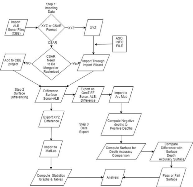
The depth raster datasets for ALB and MBES were imported into Caris Base Editor. Datasets that were provided in Caris Spatial ARchive format (CSAR) were directly imported; however, those not provided in this CSAR format were imported to Caris Base Editor through the Import Wizard as XYZ files. Difference statistics between MBES with respect to ALB surfaces were calculated for each area using the Surface Differencing tool in Caris Base Editor. For consistency in comparisons, ALB was always subtracted from MBES or ENC derived surfaces, and all depths were positive down. Difference CSARs were exported to GeoTiff raster for processing with ArcMap to analyze depth differences at each node with respect to First Order, Special Order, and Exclusive Order from Figure 2. By using the Total Vertical Uncertainty (TVU) equation (International Hydrographic Organization (IHO), 2008) and the MBES depth, a surface containing the allowable uncertainty for each node was computed at each survey order and was compared with difference surfaces referred to as “pass and fail” surfaces. A pass-fail surface determines areas that are inside and outside of the allowable uncertainties associated at each survey order based on the depth at the node. These surfaces were created for comparisons of MBES and ENC with respect to ALB. Figure 3 shows the model used to compare the depth difference values with survey order uncertainties. First the “a” and “b” values (see Figure 2), and depth value from the MBES or ENC surface were used as input into the calculation that used the TVU equation to determine the allowable uncertainty at each node. The calculation result created an allowable uncertainty raster created by replacing the depth value at each node with an absolute allowable uncertainty for that specific depth. This raster was then used to compare each node of the depth difference surface to evaluate whether the corresponding node from the depth difference surface was within the value from the allowable uncertainty raster. If the value was within the allowable uncertainty, the node was assigned a value of 1, and if it was not within the allowable uncertainty, a value of 0 was assigned to create a new surface to represent regions where depth differences meet the allowable uncertainties. Statistical analysis was conducted through Matlab to compare difference values of MBES and ENC datasets with respect to ALB. Statistics for each dataset, including the mean, median, and standard deviation at the one and two sigma levels were computed and compared with survey orders uncertainties.

Adopting the methodology for creating a TIN provided by Masetti, Faulkes, & Kastrisios (2018), an ENC derived depth surface was created for comparison to ALB. The TIN was generated in Caris Base Editor through selection and creation of a HOB file containing the ENC depth contours (DEPCNT) and ENC soundings (SOUNDG) layers. This HOB file was created through a Select by Feature Acronym and by exporting the selection to a HOB file. TINs for each ENC from Table 1 were created using this HOB file (see Figure 4). TINs included Delaunay triangles which passed through land features that required removal, as these provide false depth values. Using the Arc Map Model Builder process that uses a land feature polygon to cut out overlapping regions from the interpolated surface, all falsely interpolated values that appear over land were removed. This process is illustrated through a flow chart and images in Figure 4.


Figures 5 and 6 illustrate the process followed for comparisons and analysis of MBES and ENC with ALB, respectively.

5. Results
MBES vs ALB Comparison
Depth Differencing using MBES as a baseline in Pictou, and Mahone Bay NS show that over 90% of depth differences fall within the allowable uncertainty at each node for First Order survey (see Table 2). A pass and fail map shown in Figure 9 describes areas that are within First Order survey standards. Blue areas represent regions in Pictou that do not conform to the survey standard requirements, in this case, the First Order level. Closer investigation of satellite images in these areas suggests that dense under-water vegetation may have been an affecting factor for the ALB to penetrate through to the seafloor in Pictou (Kuus, Hughes Clark, & Brucker, 2008). Figures 11 and 12 profile graphs illustrate this possibility by ALB (red) depth values reporting much shallower than the MBES (blue) derived depths. In Mahone Bay difference values that are not within survey First Order uncertainties correspond to the blue areas in Figure 10. Local inspection through profile analysis show ALB (red) reporting depths with magnitudes of upwards to 2 metres deeper than the MBES (blue) reported depths (see Figure 11 and 12). The red box over the left tail of the difference histogram in Figure 8 shows that ALB is reporting depths that are statistically deeper than MBES approximately 8% of the time. This is of concern for safe navigation as if the ALB depths were to be incorporated directly into navigational products; this deep bias could lead to vessel accidents where published depths on navigational product are incorrect.


An additional finding with the Mahone Bay dataset was visible systematic flight-line patterns in the ALB dataset. Figure 13 illustrates a systematic bias in each flight line that can be correlated to the skew noticed by the histogram in Figure 8.

ENC vs ALB Comparison
The ENC surface contained a significantly larger amount of overlap with ALB than compared to the MBES surface, as expected (see Figures 14 and 15). Although a larger amount of coverage was provided, the depth differences reported only 61% to be within the First Order for Pictou, 31% for Mahone Bay, and 17% for Grand Manan (see Table 2). Figures 16 illustrate the pecentages for each location in blue that were within First Order uncertainties. Simplified cartography data were interpolated to a surface for comparison with high-density ALB surface leading to a conclusion that the TIN interpolation using depth contour, and depth sounding layers, does not represent the detailed seafloor between the depth values. While this result is expected, the power of the comparison methodology is in shoal detection. The region outlined by the red boxes in of the histograms of Figure 17, 18 and 19 show that 23%, 25% and 43% for the locations Pictou, Mahone Bay, and Grand Manan respectively have depth differences between ALB and ENC larger than the allowable First Order survey level with ALB reporting depths shallower than the ENCs . These regions signify where chart updates and further investigations are required to ensure safe and accurate depths are shown on navigational products.


6. Conclusions
Vertical depth differencing comparisons between ALB and MBES datasets provided a good agreement for Pictou and Mahone Bay locations, with over 90% of depth differences within the allowable uncertainties of the First Order Survey Level. Results in areas with pronounced natural seafloor attributes, such as vegetation in Pictou and slopped areas from Mahone Bay, deviated from this high percentage of agreement with most differences in these areas well outside of the allowable uncertainty ranges.
The use of ENCs was explored to interpolate a surface for comparison and assessment of ALB datasets. This comparison produced the poorest statistical results of all the vertical comparison methods, mainly due to how the surface was interpolated for the ENC layers. The ENC depth difference and assessment with ALB did, however, highlight areas to consider for ENC chart updates, providing an efficient means of focusing ALB data assessment and processing.
In summary, the most effective method for vertical assessment of ALB datasets is depth differencing with MBES datasets, but the comparison results vary greatly by region. The technological limitations of ALB are highlighted in areas of dense seafloor vegetation (Pictou) and steep slopes (Mahone Bay), but the efficiency gains are clear, especially in relatively flat, shallow areas (Pictou). Comparisons with ENCs provides an additional method for assessment, which may prove especially useful in locations where MBES datasets are not available or where focused data processing areas need to be identified for chart updates.
REFERENCES
- Costa, B. M., Battista, T. A., & Pittman, S. J. (2009). Comparative evaluation of airborne LiDAR and ship-based multibeam SoNAR bathymetry and intensity for mapping coral reef ecosystems. Remote Sensing of Environment, 113(5), 1082-1100. doi:10.1016/j.rse.2009.01.015
- Fisheries and Oceans Canada. (2017, October 24). Science – Canadian Hydrographic Service2018-2028 Strategic Directions and Quality Policy. Retrieved from http://www.charts.gc.ca/documents/help-aide/strategicdirections-orientationsstrategiques-eng.pdf
- Imahori, G., Ferguson, J., Wozumi, T., Scharff, D., Pe’eri, S., Parrish, C., . . . Aslaksen, M. (2013). A procedure for developing an acceptance test forairborne bathymetric lidar data appli cation to NOAA charts in shallow waters. NOAA Technical Memorandum NOS CS 32 , Nation- al Oceanic and Atmospheric Administration , Silver Spring, Maryland. Retrieved from https://repository.library.noaa.gov/view/noaa/2645
- International Hydrographic Organization (IHO). (2008). IHO STANDARDS FOR HYDROGRAPHIC SURVEYS. Special Publication No. 44. International Hydrographic Bureau. Retrieved from https://www.iho.int/iho_pubs/standard/S-44_5E.pdf
- Kotilainen, A., & Kaskela, A. (2017). Comparison of airborne LiDAR and shipboard acoustic data in complex shallow water enviroments: Filling in the white ribbon zone. Marine Geology, 385, 250-259. doi:10.1016/j.margeo.2017.02.005
- Kuus, P., Hughs Clark, J., & Brucker, S. (2008). Aquatic, SHOALS3000 Surveying Above Dense Fields of Aquatic Vegetation – Quantifying and Identifying Bottom Tracking Issues. University of New Brunswick, Ocean Mapping Group. Retrieved from http://www.omg.unb.ca/omg/ papers/CHC2008_PKuus120408.pdf
- Masetti, G., Faulkes, T., & Kastrisios, C. (2018). Automated Identification of Discrepancies between Nautical Charts and Survey Soundings. International Journal of Geo-Information, 7(10), 392. doi:10.3390/ijgi7100392
- Pastol, Y. (2011). Use of airborne lidar bathymetry for coastal hydrographic surveying: the french experience. Journal of Coastal Research, 6-18. Retrieved from https://www-jstor-org.proxy.hil.unb.ca/stable/29783131?seq=1#metadata_info_tab_contents
- Saylam, K., Hupp, J. R., Averett, A. R., Gutelius, W. F., & Gelhar, B. W. (2018). Airborne lidar bathymetry: assessing quality assurance and quality control methods with Leica Chiroptera examples. International Journal of Remote Sensing, 39(8), 2518-2542. doi:10.1080/01431161.2018.1430916
- Scharff, D. (2007). Application of bathymetric lidar to noaa nautical charts [Abstract]. U.S. Hydro 2007 Conference. Retrieved from http://ushydro.thsoa.org/hy07/05_01a.pdf
- UK Hydrographic Office. (2019, February 27). S-57, S-63 and S-52: The latest IHO Standards and what they mean. Retrieved from ADMIRALTY Marine Data Solutions: https://www.admiralty.co.uk/news/blogs/s-57-and-the-latest-iho-standards
BIBLIOGRAPHY
- Canadian Hydrographic Service (CHS). (2013, June). Standards for Hydrographic Surveys, 2. Retrieved from http://www.charts.gc.ca/documents/data-gestion/standards-normes/standards-normes-2013-eng.pdf
- Ellmer, W., Andersen, R. C., Flatman, A., Mononen, J., Olsson, U., & H. Ö. (2014). Feasibility of laser bathymetry for hydrographic surveys on the baltic sea. International Hydrographic Re- view, 33-50. Retrieved from https://journals.lib.unb.ca/index.php/ihr/article/view/22840/26528
- Fisheries and Oceans Canada. (2017, October 24). Science Canadian Hydrographic Service 2018-2028 Strategic Directions and Quality Policy. Retrieved from http://www.charts.gc.ca/documents/help-aide/strategicdirections-orientationsstrategiques-eng.pdf
- Goodchild, M., & Hunter, G. (1997). A simple positional accurcay measure for linear features. International Journal Geographical Information Science, 11(3), 299-306. Retrieved from http://www.geog.ucsb.edu/~good/papers/269.pdf
- Lockhart, C., Lockhart, D., Martinez, J., & Fugro Pelagos (USA) . (2008). Total propagated uncertainty (tpu) for hydrographic lidar to aid objective comparison to acoustic datasets. International Hydrographic Review, 9(2), 19-27. Retrieved from https://journals.lib.unb.ca/index.php/ihr/article/view/20821/23981
- Hare, R., Eakins, B., & Amante, C. (2011). Modelling bathymetric uncertainty.
- International Hydrographic Review Retrieved from https://journals.lib.unb.ca/index.php/ihr/article/view/20888/24048
- McKenzie, C., Gilmour, B., Van Den Ameele, E. J., & Sinclair, M. (2001). Integration of LIDAR Data in CARIS HIPS for NOAA Charting. Paper presented at 6th Annual International CARIS Users’ Conference. San Diego,United States. Retrieved from http://citeseerx.ist.psu.edu/viewdoc/download?doi=10.1.1.549.3603&rep=rep1&type=pdf
- National Oceanic and Atmospheric Administration. (2016). Integration of U.S. Army Corps of Engineers airborne LIDAR bathymetry (ALB) survey data into NOAA’s processing workflow. Retrieved from https://repository.library.noaa.gov/view/noaa/16916/noaa_16916_DS1.pdf
- The University of New Hampshire. (2018, October 24). CUBE. Retrieved from Center for Costal and Ocean Mapping Joint Hydrographic Center: http://ccom.unh.edu/theme/data-processing/cube
- Witmer, J. D., Imahori, G., Aslaksen, M., Gonsalves, M., Berkowitz, E. E., & Shachak,
- P. (2016). Integration of U.S. Army Corps of Engineers Airborne Lidar Bathymetry (ALB) survey data into NOAA’s processing workflow. NOAA Technical Memorandum NOS CS 36,Silver Spring. doi:http://doi.org/10.7289/V5/TM-NOS-CS-36
AUTHORS BIOGRAPHY
Michel Leger is a Multi -Disciplinary Hydrographer for the Canadian Hydrographic Service at the Bedford Institute of Oceanography. Michel obtained a B.Sc.Eng. in Geomatics from UNB in May 2019. Michel held several positions as an Undergrad Research Assistant with the Ocean Mapping Group at UNB. In 2017 Michel held a research award from the National Science and Engineering Research Council under the supervision of Dr. Emmanuel Stefanakis and Dr. Heather McGrath focusing on accuracy comparisons of Web Elevation Services as part of UNB’s flood mapping research. Currently, Michel’s research interests are in automation and standardization of hydrographic processing workflows using Python Programming. Email: Michel.leger@dfo-mpo.gc.ca
Jia Gong is currently a Technical Support Consultant at Teledyne CARIS. He earned a Bachelor of Science in Engineering from the University of New Brunswick (UNB), where he was proactively involved in the UNB’s Ocean Mapping Group under the supervision of Dr. Ian Church. He was the recipient of the Canadian Hydrographic Association Award in 2018. Jia had also worked as Student Hydrographer for nearly four months in 2018, where he devised and developed a MATLAB-based solution for numerically assessing the Airborne Lidar Bathymetry datasets. Under the supervision of Dr. Emmanuel Stefanakis, he realized a comparative quality assessment of the crowdsourced geographical datasets relative to the officially released ones in 2017. His current research interests are in automated data processing and assessment, Airborne Lidar Bathymetry, and crowdsourced geographical information. Email: jason.jia.gong@gmail.com
Dr. Ian Church is an Assistant Professor in the Department of Geodesy and Geomatics Engineering at the University of New Brunswick, where he leads the Ocean Mapping Group. Before starting at UNB in 2016, he was an Assistant Professor with the Hydrographic Science Research Center at the University of Southern Mississippi. He received his B.Sc.Eng, M.Sc.Eng and Ph.D. from UNB while working under the supervision of Dr. John Hughes Clarke. His current research interests are in automated data processing, integrating numerical hydrodynamic modelling with ocean mapping, marine habitat mapping, and acoustic water column interpretation. Email: ian.church@unb.ca