1 Introduction

A local chemical company operates evaporation ponds in their Dead Sea site located in the southern basin of the Dead Sea in Israel. These ponds, fed by a feeder canal from the northern basin, are very shallow, hypersaline water bodies of extremely high temperatures, enhancing rapid evaporation and minerals crystallization. Operation of these ponds demands frequent hydrographic surveying to determine chemical harvesting requirements and results and to calculate required water replenishment volumes.

Until recently, all surveying was conducted either by a Land Surveyor using real-time kinematic (RTK) GNSS or single beam echo sounding, depending upon the depths of the ponds. Both methods produce discontinuous data with limited coverage, requiring much interpolation to fill the data gaps. In a very heterogeneous environment with mineral crystals of various sizes and shapes, randomly spread over the pond bottoms, interpolation results in relatively low accuracy survey products.

This paper describes and elaborates on a three-day campaign, during September 2024, to survey three ponds and a section of the feeder canal using a multi beam echo sounder (MBES) survey system mounted on a small, flat bottomed boat.

2 Aim

The purpose of the survey project was to evaluate the feasibility of using a MBES system in these extreme conditions and, if feasible, to determine whether the advantages in using this method of surveying are cost effective. In addition, and depending upon the final results, the project aimed to produce insight into the methodology of such a survey and any required emphasis on certain aspects to achieve desired results.

3 The project sites

The Dead Sea, lying between Israel and Jordan, is divided into two basins. The northern basin, the larger in area, reaches depths up to approximately 300 m. In 2006, a comprehensive MBES survey was conducted in the northern basin using an ELAC 1050 50 kHz MBES. At the time of that survey, the Dead Sea surface was measured at -421 m below the Mediterranean mean sea level (MSL; Beaudoin et al., 2011).

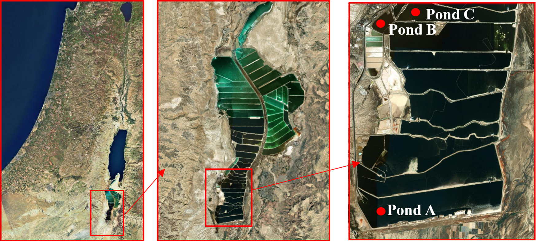
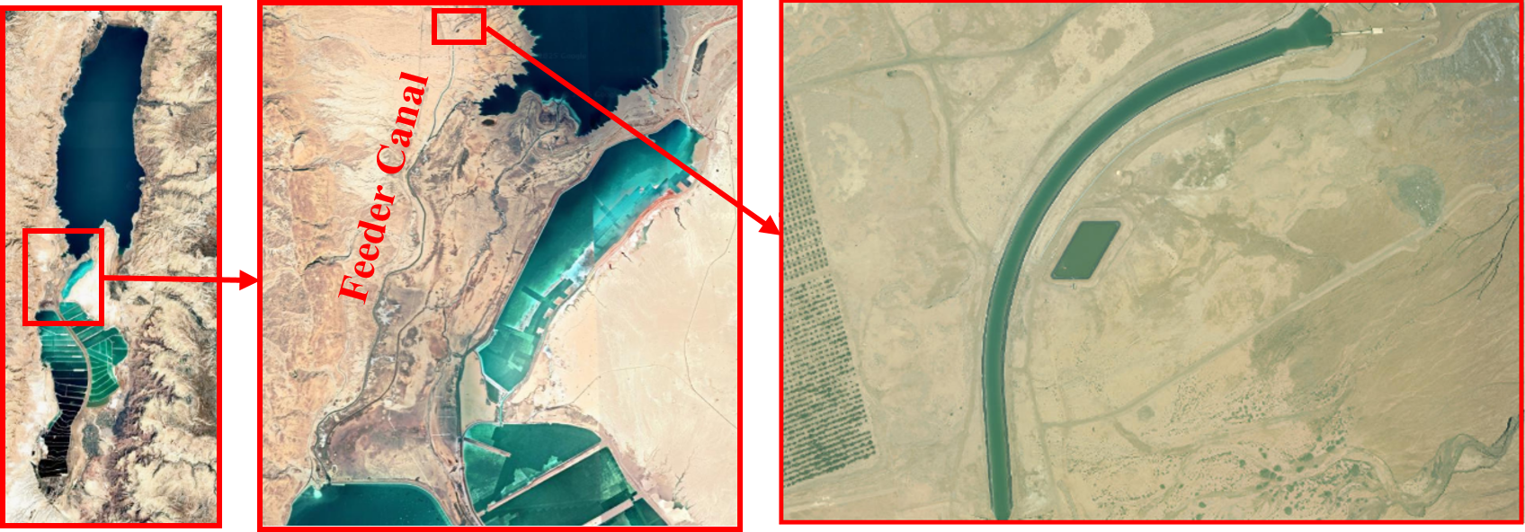
The southern basin consists today of a number of interconnected evaporation and waste disposal ponds, operated for harvesting various minerals. Fig. 1 shows the general area and the evaporation ponds. On the left is a general picture of Israel and the Dead Sea, in the center is an enlargement of the ponds in the southern basin and on the right is an enlargement where the three evaporation ponds, A, B and C, involved in this study, are shown by red dots. In Fig. 2 one can see the feeder canal and in the enlargement the section surveyed in this study.

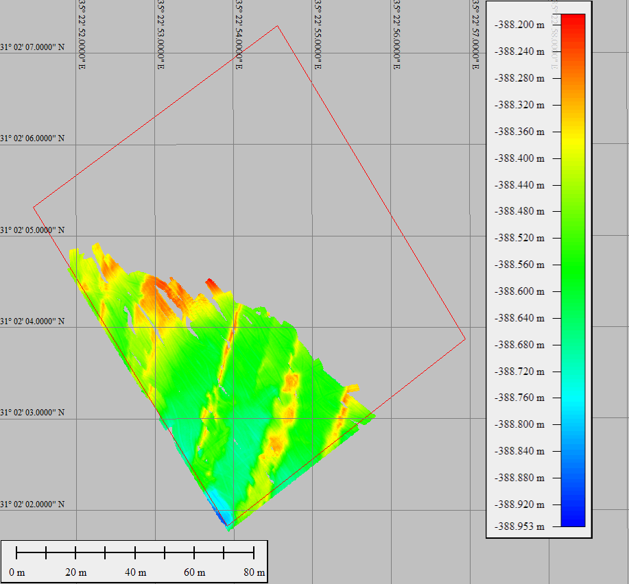
In each pond a small area was designated for surveying for this feasibility study. In pond A the area surveyed covered 7,500 m², in pond B the area surveyed was 16,800 m² and in pond C the area planned for surveying was 12,500 m^2. However, in pond C only 4,850 m² were actually surveyed due to very shallow depths inaccessible by boat. Fig. 3 shows the area actually surveyed relative to the planned area in pond C.

Evaporation pond A has depths of about 2 m, measured water temperature of 38.8 °C, salinity ranging between 350 PSU (Practical Salinity Units) on the surface to 359 PSU on the bottom, water density averaging 1,286 kg/m³ and sound speeds of 1,870 m/s at the surface to 1,878.7 m/s on the bottom.

Evaporation pond C has depths less than 1 m, measured water temperature of 38.8 °C, salinity ranging between 377 PSU on the surface to 384 PSU on the bottom, water density averaging 1,313 kg/m³ and sound speeds of 1,897 m/s at the surface to 1,899.6 m/s on the bottom.

Mud and waste pond B has depths of up to 1.7 m, measured water temperature of 38.8 °C, salinity ranging between 375.7 PSU on the surface to 377 PSU on the bottom, water density averaging 1,310 kg/m³ and sound speeds of 1,895.7 m/s at the surface to 1,897 m/s on the bottom.

The feeder canal, surveyed near the intake station on the shores of the northern Dead Sea basin, has depths varying according to the pumping schedule. Depths during the survey reached up to 6m, measured water temperature of 34.87 °C at the surface to 34.28 °C on the bottom, salinity averaging 299.9 PSU, water density averaging 1,240 kg/m³ and sound speeds of 1,820.5 m/s.

Table 1 summarizes the Dead Sea ponds characteristics. The SVP data and graphs of the depth-dependent sound speeds and salinities are given in Fig. 4.

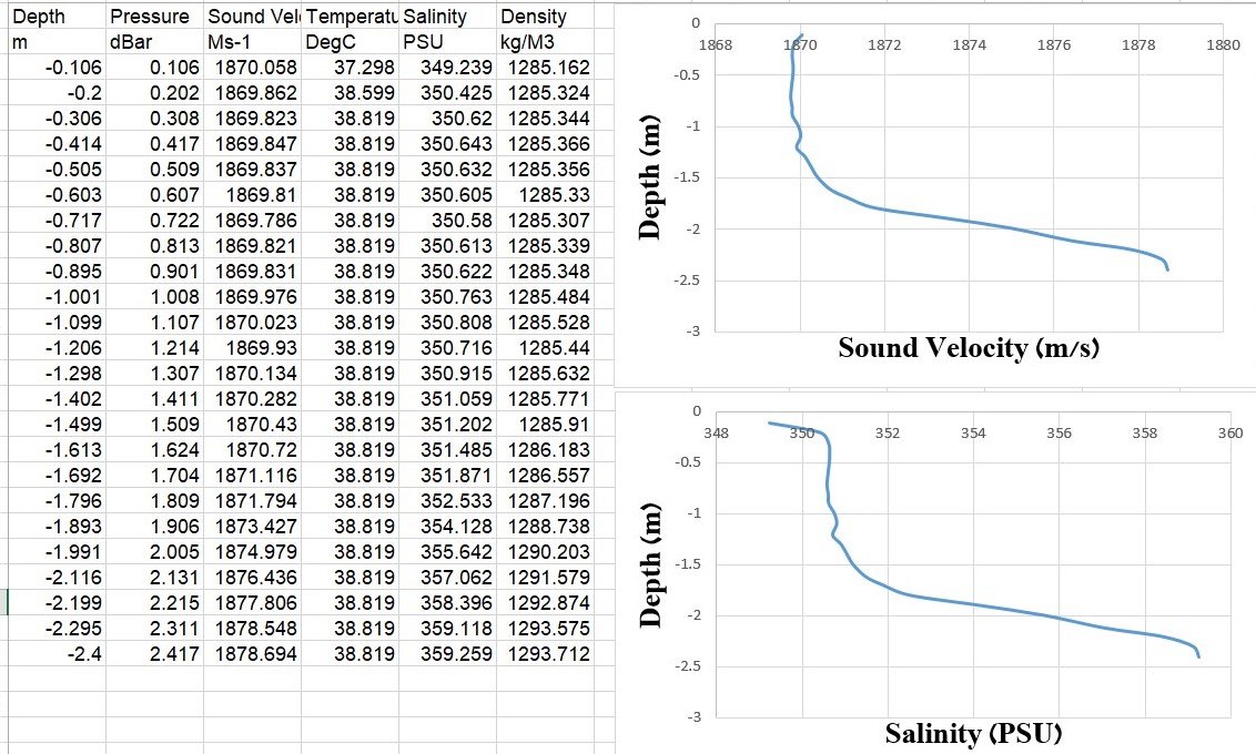
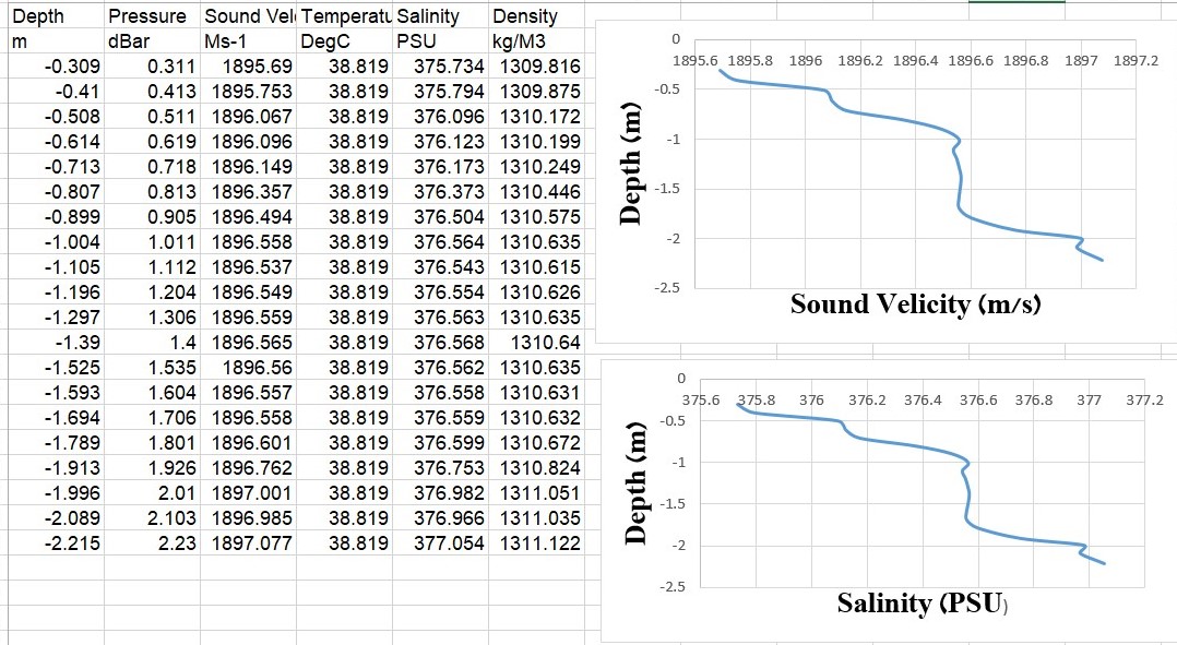
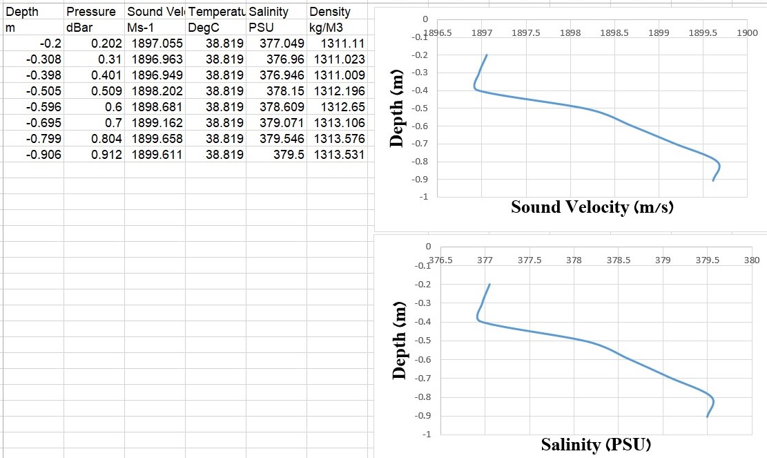
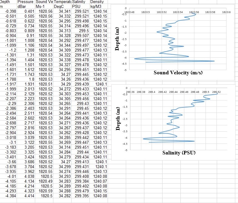
It is clearly evident that in the ponds the salinity increases significantly towards the bottom, consequently resulting in an increase in sound speed. Water temperature does not change significantly due to the very shallow depths so the major influence on sound speed is clearly the salinity. In the feeder canal on the other hand salinity and water temperature have little variation with depth, thus the sound speed has very small and insignificant changes with depth – varying only 0.14 m/s between the surface and 4.5 m depth.

Note that density was calculated according to salinity measurement of the Valeport Swift SVP, using the EOS80 formula suited for regular sea water. The Valeport profiler specifications claim an accuracy of 0.01 kg/m³ and a resolution of 0.001 kg/m³. Dead Sea water, having a larger variety of minerals than regular sea water, is expected to have a higher density than that calculated.

As the title of this paper indicates, these are extremely challenging conditions for conducting a MBES hydrographic survey. Measuring calibration parameters to input into the survey equipment requires instruments suitable for these high salinities and sound speeds. Most instruments are calibrated for regular sea water. For example the AML – 3 LGR SVP (500 m) measures sound speeds between 1,375–1,625 m/s. In addition the very shallow waters and salt mushrooms or muddy bottoms demand much caution during the survey, both for safety reasons and reliable data collection, with noise and acoustic reverberation prevalent.

4 Required results

The main incentive for this project was to obtain a continuous map of the ponds with the highest accuracy possible, in a cost-effective manner. Accuracy would in this case refer to the depiction of the ponds’ floors, including both depth relative to a reference level and position, in order to determine mineral harvesting or water replenishment requirements. Certainly, IHO S-44 standards, pertinent mainly though not entirely to navigation, are not relevant in this case with the project being more of an engineering issue rather than one intended for navigation. In addition, depths relative to the ponds’ surfaces are more of interest for the site operators than absolute depths, reduced to a chart datum such as the Israel Land Survey Datum (I.L.S.D). Tides are naturally irrelevant in these small ponds.

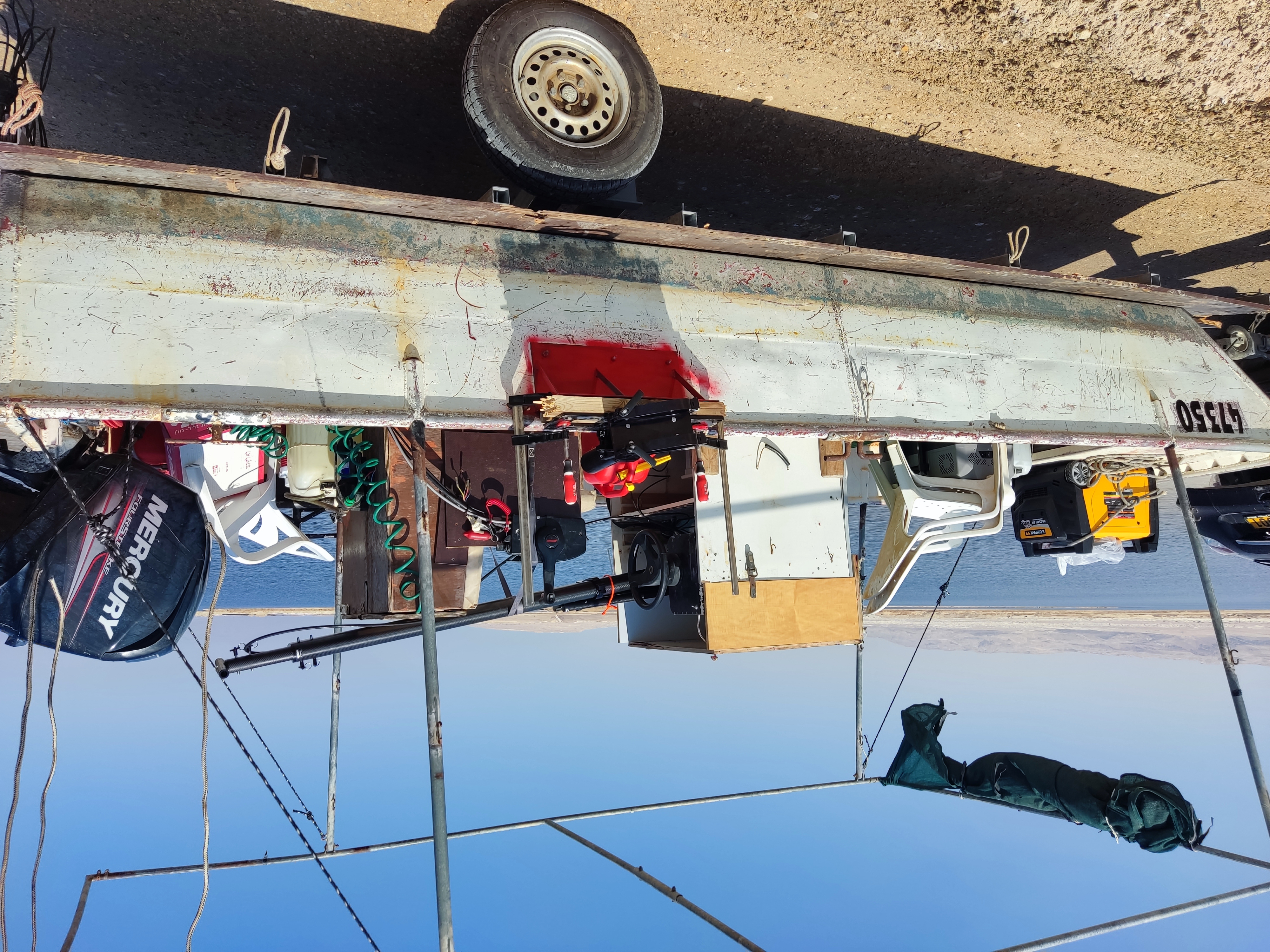
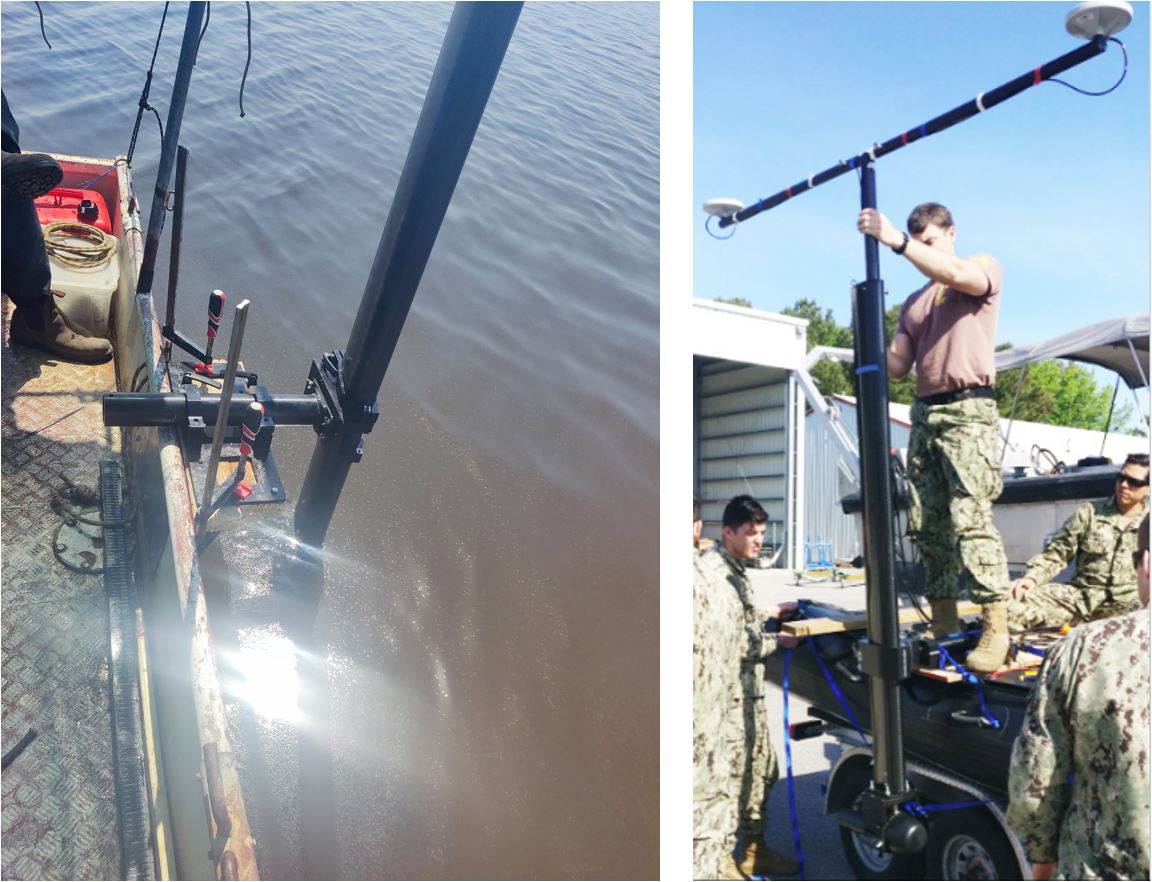
With this in mind relevant procedures were undertaken, considering restraints due to the extreme environment, to achieve the highest position and depth accuracy and complete coverage of the ponds’ floors. For example, during the equipment installation, the use of a portable refrigerator box for all the topside electronics was necessary in order to avoid overheating (air temperature at the site was around 40 °C – certainly extreme). A Patch Test was not conducted since one would be impossible in such shallow waters and the effects of orientation offsets, usually small, could be considered negligible. The Norbit iWBMS suite comes with the IMU mounted on the transducer, eliminating any concern regarding blatant equipment installation errors. Maximum precaution was taken to install the equipment with the best orientation and in the most stable manner possible. The installation of the Norbit Portus Pole, attached to a rigid bracket over the side of the boat, shown in Figs. 5 and 6, contributed to substantially reducing all angular offsets of the IMU and the attached MB transducer.

In addition, requiring depths relative to a practical reference level for operational purposes in the ponds, together with the frequent GNSS spoofing during the campaign, led us to conduct the survey in the following method. Transducer draft was measured at the beginning of each survey and added to the measured and calculated depths below the transducer (DBT) to provide instantaneous depths below the ponds’ surfaces (DBW). At the same time, elevations of the ponds’ surfaces (negative of course) were recorded from the local tide staffs which are geodetically related to the I.L.S.D. level through a Survey of Israel (SoI) benchmark in the area. Thus, by combining the three measurements, DBT, draft and tide staff reading, the ponds’ bottom surface was obtained relative to I.L.S.D for comparison with the land surveyor’s GNSS RTK measurements reduced also to I.L.S.D using the SoI’s ILUM 2.0 model. In this way we obtained both a practical output for the ponds operators as well as output for quality assessment and accuracy evaluation.

5 Equipment used

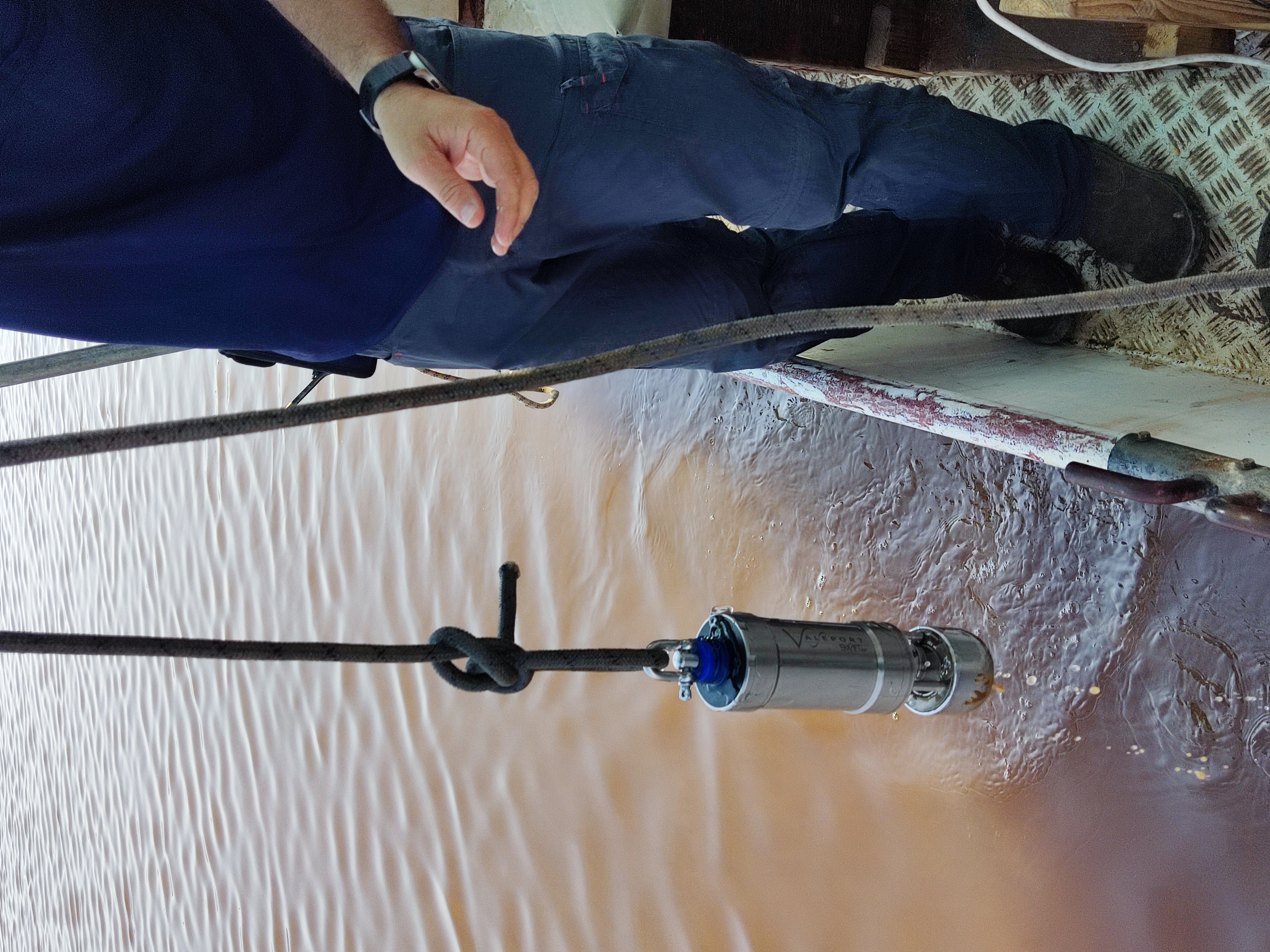
For this project we used the Norbit iWBMS survey equipment with frequencies between 200–700 kHz, mounted over the side using a Norbit Portus Pole. The iWBMS comes with a SBG Equinox GNNS/INS embedded system to measure pitch, roll and heave mounted on the transducer and, understanding that the unusual environment would require irregular measuring equipment, a high sound speed calibrated sound velocity sensor (SVS) to measure water sound speed at the sonar head. Navigation and heading data were collected with two GNSS antennae mounted on top of the Portus Pole. In addition, a Valeport sound velocity profiler Swift SVP, calibrated to measure sound speeds up to 1,900 m/s, was used in each survey area prior to commencing the survey.

Figs. 5, 6 and 7 show the survey boat, the pole mounting of the iWBMS and the GNSS antennae and the SVP used.

Data acquisition was obtained on board using QPS Qinsy software and data processing in the office using Qimera.

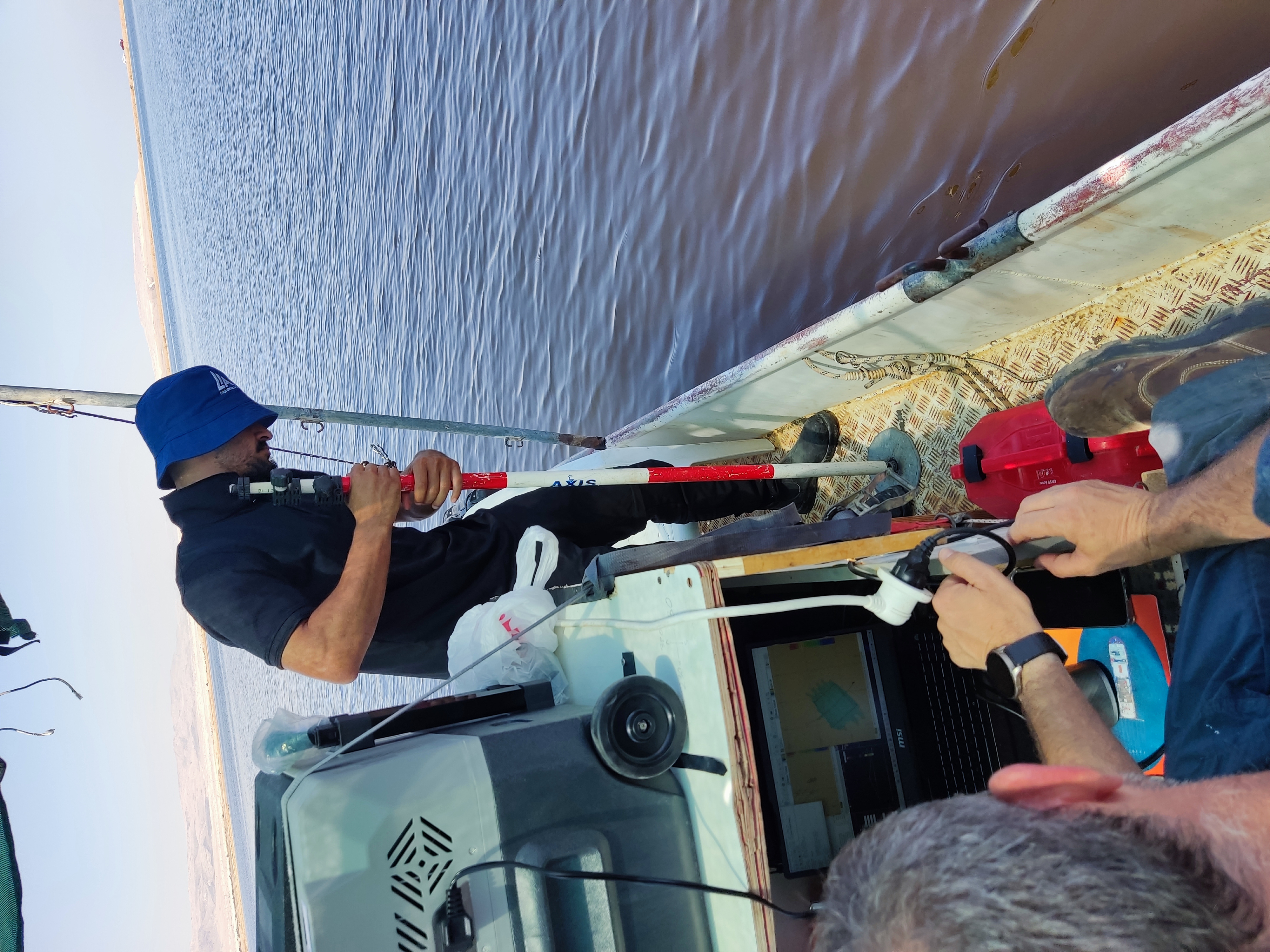
Control and quality assessment was done by comparing the processed data to point measurements in each area, taken by a Certified Land Surveyor using Leica RTK GNSS. Considering the possibility of soft sediments in some of the ponds, a 7.5 cm radius round disk was attached to the bottom of the survey pole in order to avoid penetration below the sediment surface. Fig. 8 shows the disk attached to the surveyor’s pole.

6 Method

The first day of the project, on September 8^th 2024, involved mobilization of the boat, preparing and installing the equipment. Heading was calibrated during the GNSS Azimuth Measurement Subsystem (GAMS) setup with position calculations running eight shaped maneuvers until the heading solution reached the system accuracy threshold. Once this was completed the survey team commenced to the feeder canal. After measuring transducer draft using a measuring tape, taking an SVP cast and entering the results into the acquisition software (QPS Qinsy), the team began surveying along 1 km of the canal. The swath angle was set at 150° in order to maximize coverage due to extremely shallow water depth and after testing several frequencies, transducer acquisition frequency of 400 kHz was chosen as it had the best signal to noise ratio. Since it is narrow, only two survey lines were run along the canal, ensuring a large percentage of overlap. Ten RTK GNSS measurements were taken by the Land Surveyor along the survey lines for comparison.

During the canal survey pumping took place changing the absolute water level from time to time. Understanding that the purpose of the survey in this area was not to measure depths, the emphasis was placed on getting a high-resolution picture of the plastic lining on the canal floor. Severe GNSS spoofing during the survey, did not allow the use of RTK height as a reference, hence absolute depths along the canal were unobtainable and the relative depths were used only to produce a picture of the canal’s floor. Using the 400 kHz option with a wavelength less than 5mm enabled obtaining excellent resolution. The GNSS spoofing naturally affected the position of the soundings as well, but this was corrected by moving the final DEM into place manually, using conspicuous features along the canal as anchors for the necessary horizontal translation.

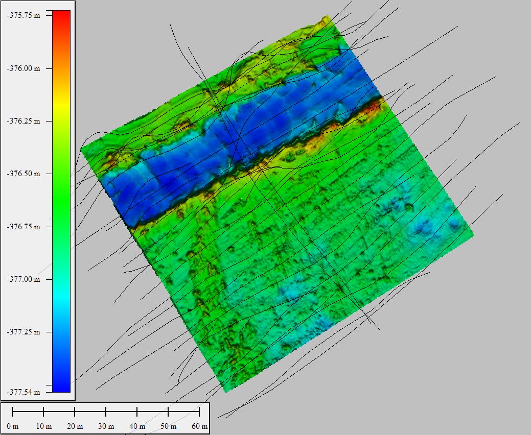
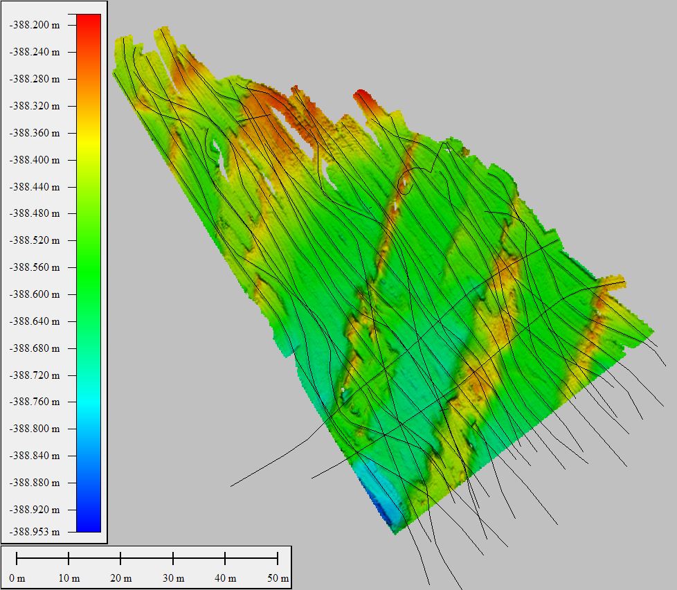
The following day, September 9^th, began by deploying the survey boat to pond A at the southern end of the southern basin. After measuring transducer draft, taking an SVP cast and entering the results into the acquisition software, the team began surveying along the main survey lines, in a NE–SW direction. Line spacing varied between 3.3 m and 6.5 m, ensuring adequate overlap. Swath angle was 150° and frequency 200 kHz as it had the best signal to noise ratio after testing several frequencies. Thirty-three main survey lines were run with two perpendicular cross check lines, covering 2.4 NM during 1 hour and 20 minutes of surveying at 1.8 knots. After completing the MBES survey, sixteen GNSS RTK measurements were collected by the Land Surveyor, spread around the surveyed area. Fig. 9 shows the survey lines run in pond A, overlaid on the color-coded bathymetry.

The third day of the project, September 10^th, began with the survey boat deployed in the mud and waste pond B. Once again, the transducer draft was measured and an SVP cast taken. Nineteen main survey lines were run in a N–S direction with another two perpendicular cross check lines. Line spacing varied between 5 m and 10 m ensuring adequate overlap. Swath angle was 150° and frequency alternated between 200–400 kHz with changes made on board according to the quality of the raw data collected. The frequency changes were made due to extreme water density variations in the survey area, mainly due to different water composition in the dredged canal bottom. The survey lines overall length was 2 NM and the survey took one and a half hours at 1.33 knots. After completing the MBES survey, only three GNSS RTK measurements were taken for quality assessment due to GNSS spoofing during the land survey. Fig. 10 shows the survey lines run in pond B, overlaid on the color-coded bathymetry.

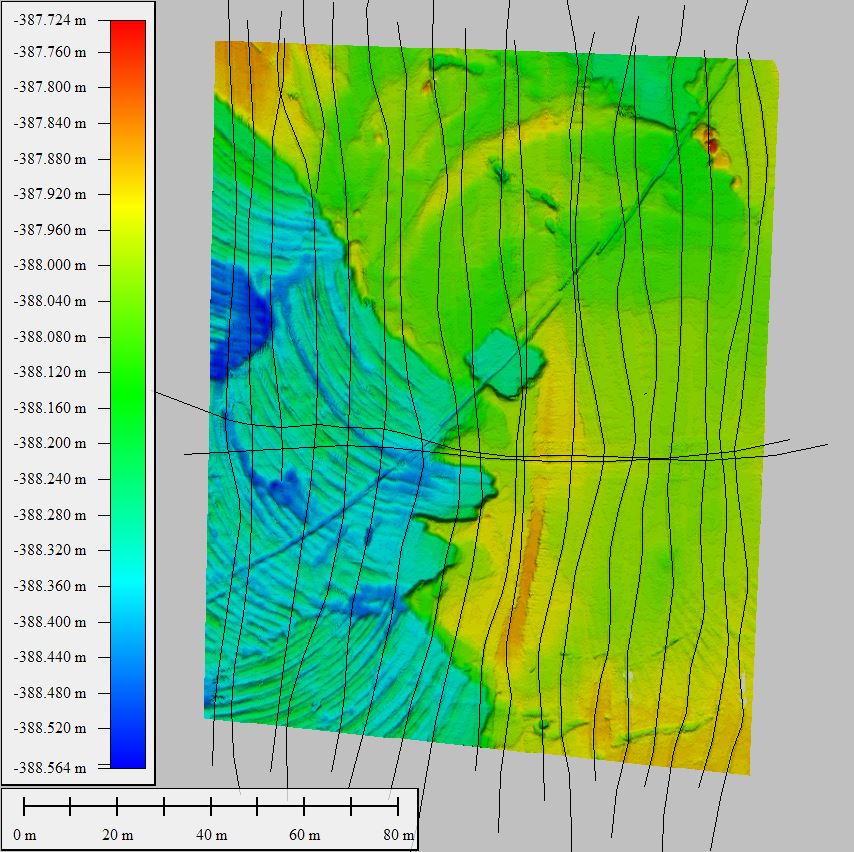
Then the survey boat was transferred to pond C where twenty-four main survey lines were run in a NW–SE direction with another two perpendicular cross check lines. Line spacing varied between 2.2 m and 4.7 m ensuring adequate overlap. Swath angle was 150° and once again the frequency was alternated between 200–400 kHz as deemed pertinent according to the quality of the raw data collected. This was done according to the reasons explained in the previous paragraph, only this time an additional reason was changes in the water composition in the survey area resulting from diverse water densities and temperatures which created some hot and dense water cells within the survey area. The survey lines overall length was 1.3 NM and the survey took one hour at 1.3 knots. After completing the MBES survey, five GNSS RTK measurements were taken for quality assessment. Fig. 11 shows the survey lines run in pond C, overlaid on the color-coded bathymetry.

The RTK GNSS validation measurements undertaken by the land surveyor used the ellipsoid height and the survey of Israel’s national undulation model, ILUM 2.0, producing elevations relative to the Israel Land Survey Datum (ILSD). Naturally in the Dead Sea area all elevations are negative.

7 Data processing

After each survey day, raw *.db files were imported into QPS Qimera for preliminary processing and data evaluation using a 20 cm cell size dynamic surface. A SVS – SVP comparison was conducted and IMU data loaded for navigation and attitude post processing in order to achieve better results.

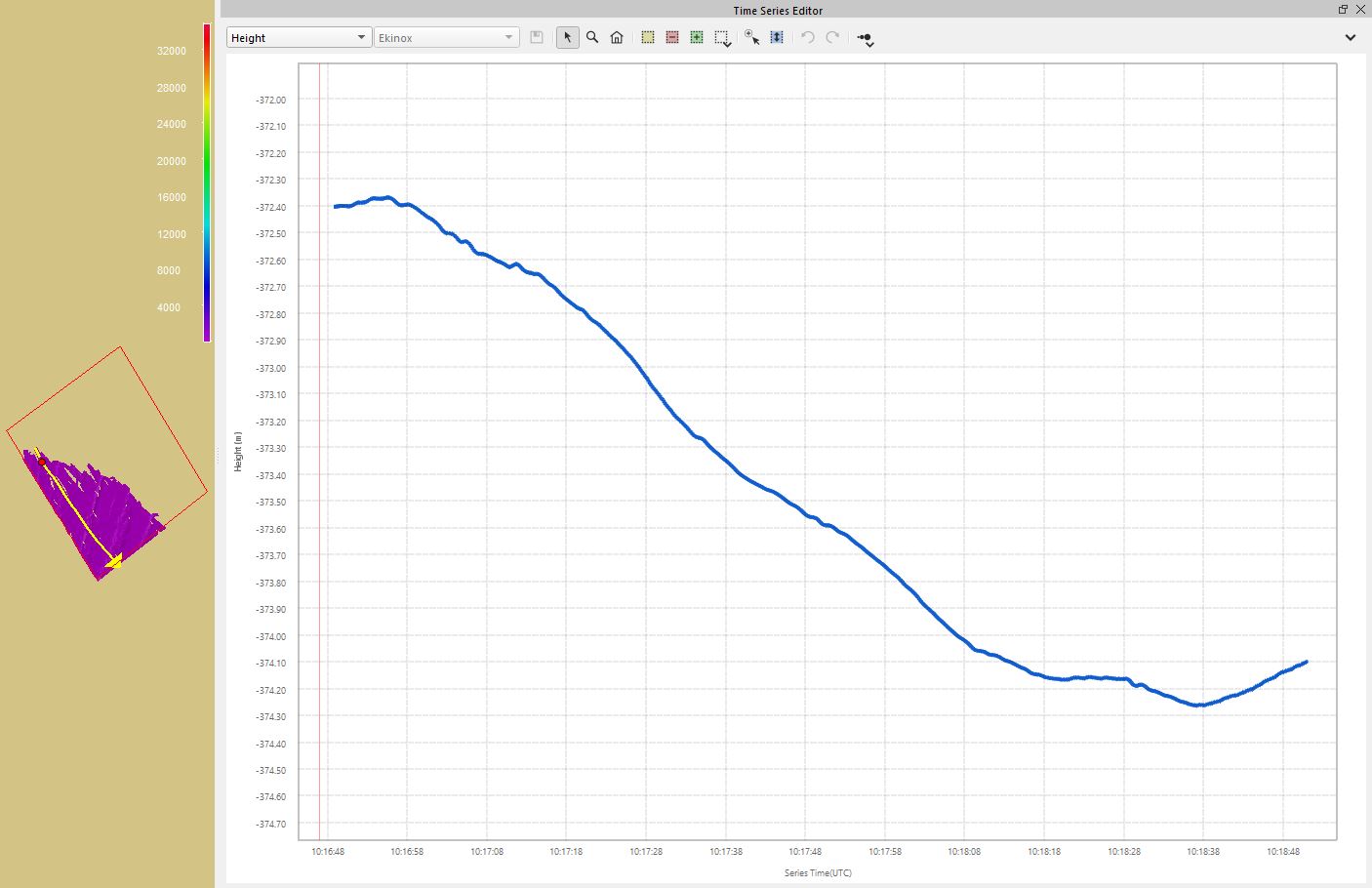
Then after approval of data quality and coverage the data was backed up on two SSD HDD for additional processing in the office where each survey area was deeply cleaned using the cloud point slice editor along with a 3D view of same data. During data processing, we noticed some GNSS spoofing which could cause an ERS survey to have significant error variations of the Z-values in some survey lines (Fig. 12). Therefor it was decided to use sonar depth along with draft and tide staff data instead of RTK height. Elevations were then reduced to ILSD ILUM2 using local tide staff gauges in each pond and UTC time.

The difference between the ellipsoidal height at the beginning of the line and that at the end of the line a couple of minutes later, reached up to 2 m. The survey line is displayed on the map to the left (Fig. 12).

Each dynamic surface was then exported as an ASCII *.xyz file and loaded into Blue Marble’s Global Mapper program where it was cropped and transformed to local CRS and exported in the same format as final processed datasets.

8 Results

Post processing involved cleaning the data and preparing a 20 cm grid map of each area. In Table 2 is a summary of the results obtained in the ponds.

9 Data analysis

The data was analyzed by visual comparison of the main survey lines with the cross sections at the intersections. In addition, the MBES 20 cm gridded output was compared to the land surveyor’s RTK GNSS measurements where available. Where prominent features were observed, their interpretation was validated with the site operators in charge of the ongoing works.

9.1 Pond A

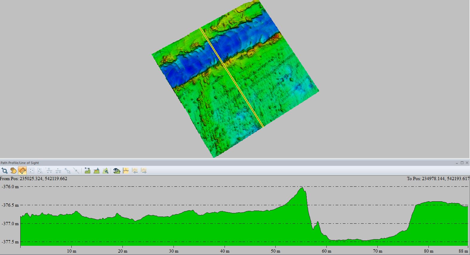
In pond A, a channel, 19 m wide and 1 m deep, is clear evidence of previous harvesting in the area. Fig. 13 shows this channel in a top view and a cross section.

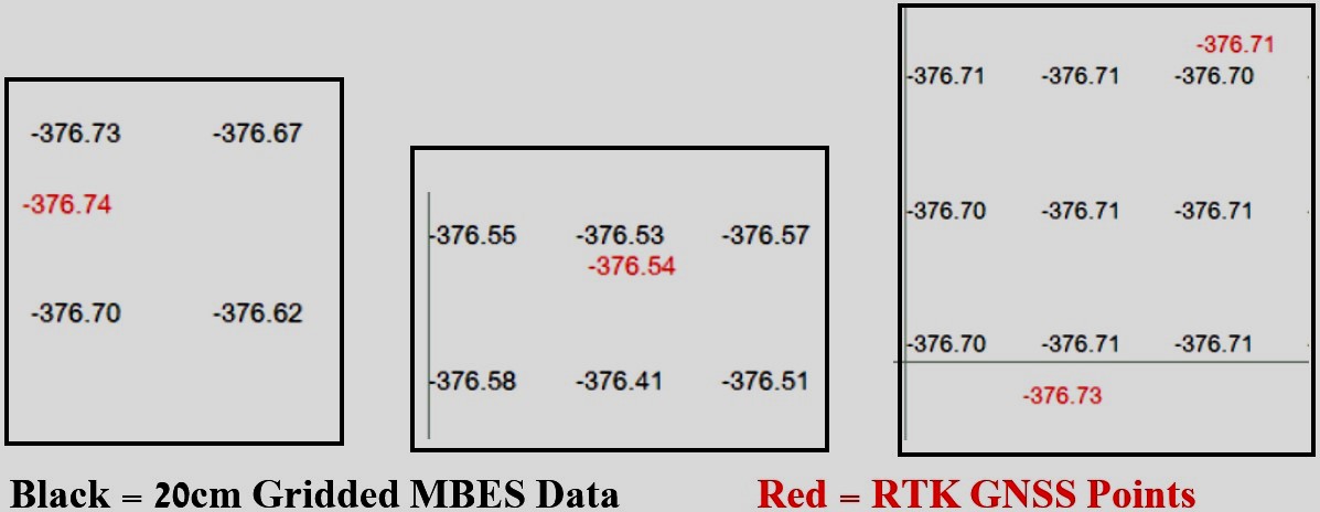
Comparison between the MBES output and the RTK GNSS points shows differences on the order of one or two centimeters, as demonstrated in Fig. 14.

9.2 Pond B

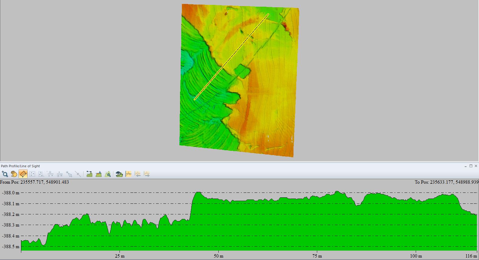
This pond with a muddy bottom was surveyed at 400 kHz in order to obtain the highest resolution possible. Fig. 15 clearly demonstrates signs of dredging in the “deeper” area to the south-west and the smoother “shallower” area to the north east where dredging and waste extraction had yet to be conducted.

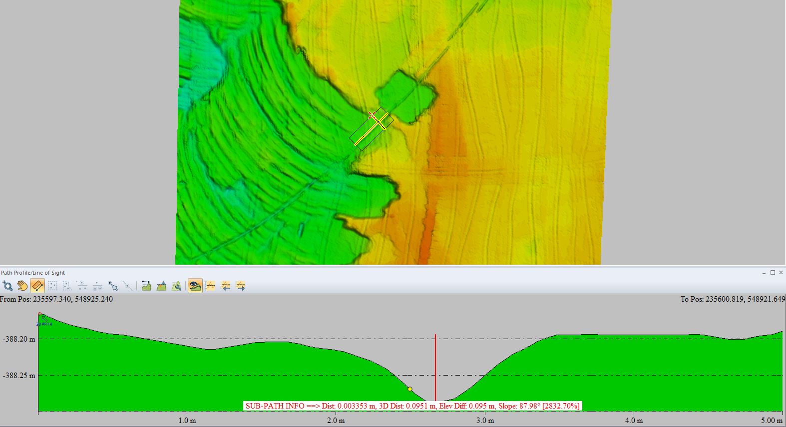
Another feature observed here is a shallow 9 cm furrow, remanence of a cable that lay on the muddy bottom which was removed some time prior to the survey (Fig. 16).

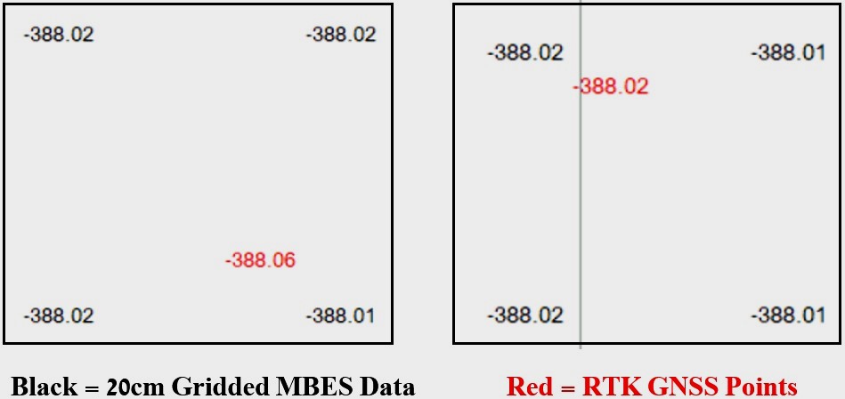
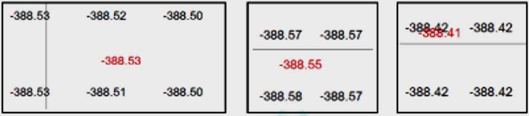
In this pond the land surveyor had difficulty discerning exactly when the disk attached to his survey pole reached the bottom. When raising the disk out of the water after taking the measurement, mud covering it indicated that the measurements were taken a little below the surface of the mud. This was validated in the comparisons with the MBES data which were usually shallower than the RTK GNSS points, as shown to the left in Fig. 17 below. In some areas however, the bottom was a little more consolidated and the data was compatible, as shown to the right in Fig. 17.

9.3 Pond C

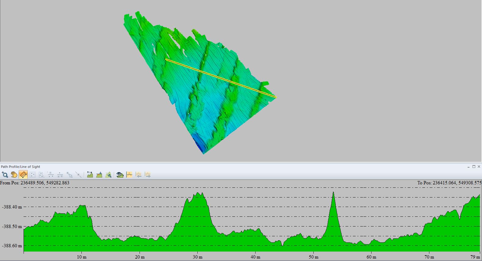
This pond was only partially surveyed due to part of the planned area being inaccessible by boat. Salt harvesting is evident in Fig. 18 with furrows 20 m wide with depths between 25 cm and 30 cm. The remnant salt ridges running parallel in a NE–SW direction are clearly seen. As in pond A, the MBES – RTK GNSS comparisons show excellent correlation, with differences of 1–2 cm (Fig. 19).

9.4 Feeder canal

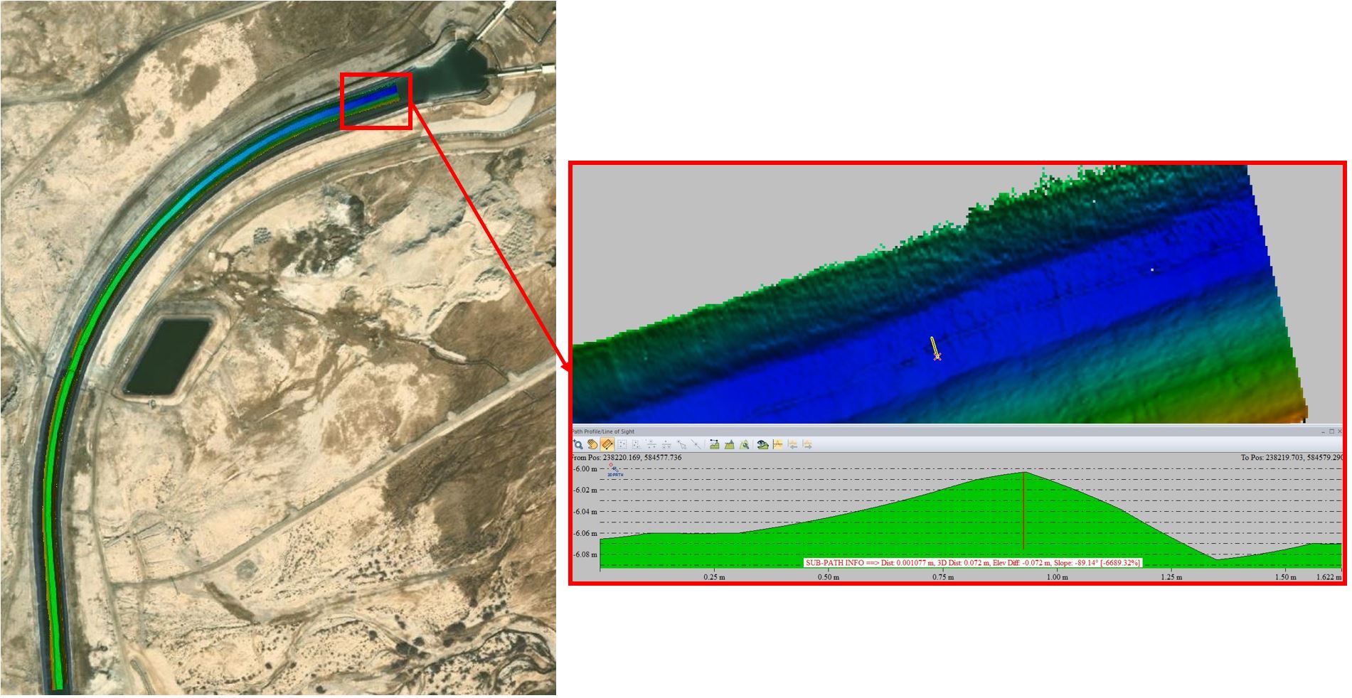
As mentioned earlier, the feeder canal was surveyed with the intention of providing a high-resolution picture of the canal’s bottom, rather than bathymetry which varies according to the pumping schedule.

Near the intake pumping station P9 close to the shore of the Dead Sea northern basin, the maximum depth reached approximately 6m. Here folds in the plastic sheets lining the bottom are evident, as shown in Fig. 20. These folds change the depths on the order of 6 cm.

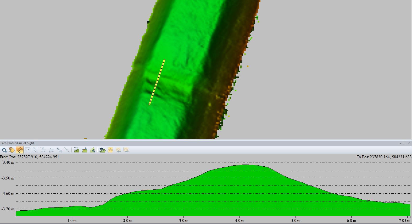
In another area, approximately 600 m from the beginning of the canal opposite to the water reservoir, a 30 cm protrusion runs across the entire canal width. This protrusion, demonstrated in Fig. 21, correlates with a concrete beam used to anchor the plastic sheets.

10 Conclusions

The extreme conditions of this project – very shallow, highly saline, warm water with either a very soft or a crystallizing hard, heterogeneous bottom – posed many potential problems. In order to ensure required results, the following procedures needed special attention:

• Choice of suitable vessel and equipment capable of working in this extreme environment.
• Equipment alignment during installation – considering no Patch Test done.
• SVP measurements up to 1,900 m/s conducted in each area, as deep as possible and as close to the bottom as possible, entered into the data collection program prior to beginning each survey.
• Slow survey speed to obtain as much overlap and redundancy as possible – required also for safety in shallow, small ponds.
• Small line spacing distance, considering swath angle used and surveyed area depth, to ensure sufficient overlap.
• Careful real time monitoring of data collection along the survey lines to ensure continuous overlap and no data gaps.
• Continuous monitoring of data quality, including GNSS fixes, throughout the survey – stopping data recording when raw data considered contaminated with errors.
• Frequency adjustment during the survey to obtain the highest resolution and best results possible.

However, certain elements of MBES hydrographic surveying, complex, if at all possible, proved to be negligible and unnecessary in these conditions. These elements, not addressed in the survey, include:

• Patch Test calibration of the equipment – small misalignment angles produce negligible errors in such shallow depths. For example, a 1° angular roll offset would result in a 0.3 mm depth error and 3.5 cm horizontal error at a nominal depth of 2 m in the nadir and 3 cm depth error and 1.7 cm horizontal error at an outer beam of 60°.
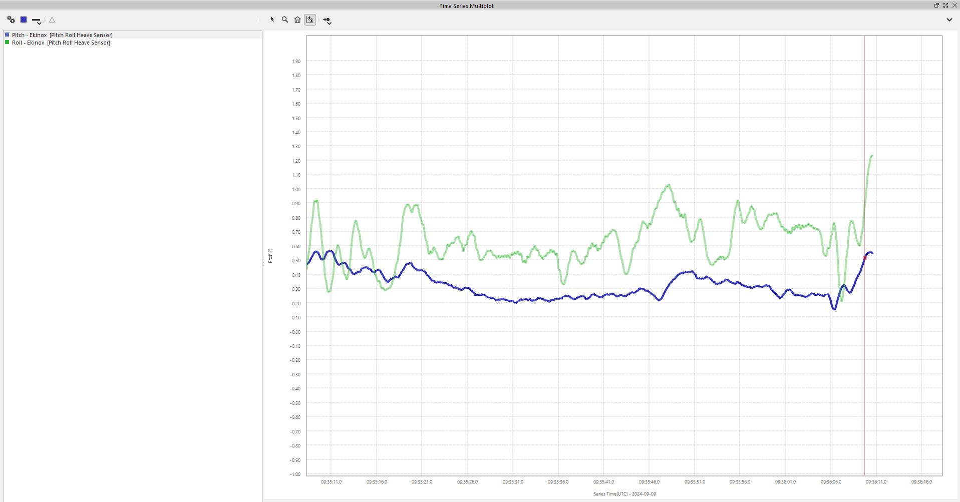
• Pitch and roll angles and heave values are very small in a pond limited in size where waves do not develop – their impact on the final results in such shallow waters are negligible (Fig. 22).
• Horizontal offset measurements – having the GNSS antennae placed on the pole above the transducer makes only the vertical offset calibration relevant. The horizontal offset is determined by the Portus Pole manufacturer.
• Draft measured in each area on each day was the same despite water density differences, probably due to the flat bottomed, small boat.

The results of this project clearly show that MBES surveying in the extreme conditions of evaporation ponds is feasible. Careful attention to critical aspects of hydrographic surveying is essential to obtain required results, while other aspects, less relevant in this case, may be overlooked.

The results show a continuous DEM of the evaporation ponds’ substrates, portrayed on a 20 cm grid in this case. In addition, the artificial lining of the feeder canal was clearly seen in the data produced after post processing.

This project gave us an insight into the implications involved in using this technique to monitor the evaporation ponds and the feeder canal. The surveys conducted covered small areas in each pond. Understanding that the chemical company would probably need larger scale surveys, with more extensive coverage in each pool, this project will enable them to estimate costs and time frames for future surveys.

References

Beaudoin, J., Sade, A., Schulze, B. and Hall, J. K. (2011). Dead Sea Multi-beam Echo Sounder Survey. Hydro International, 15, pp. 21–23.