


Abstract
1 Introduction
Accurate and reliable DBMs are needed for safe navigation in waterways. This is especially important for Germany – a leading global economic and export nation that relies heavily on its inland and maritime shipping routes to connect industrial hubs to seaports and ensure access to international markets. Its waterways, which connect the North and Baltic Seas and are central to Europe, are vital to the European waterway network, supporting trade and transport safety (BFG, 2013). Nowadays, with the capabilities of sonar-based systems such as MBES, it is possible to sample underwater topography in high spatial resolution and density. These systems measure both location and depth, generating Point Cloud (PC) comprising millions of points in a short time. Although high-resolution measurements are associated with greater detail and raise expectations regarding the detection of fine structures and higher accuracy, assumptions about the precision of such data can be misleading, as each measurement is subject to both vertical and horizontal uncertainties. The International Hydrographic Organization (IHO) provides guidelines to ensure safety and guarantee a minimum level of accuracy for users in order to standardize the quality of DBMs (IHO, 2022).
To create DBMs, we rely on raw measurements from which outliers have been removed. However, this process makes it difficult to produce a high-quality DBM because the source data are not always as accurate as required. Bathymetric measurement uncertainty depends on both the survey system and survey conditions. A survey system is, in essence, a multi-sensor system composed of several sensors (e.g., MBES, IMU, GNSS, etc.). The error budget is influenced by various factors related to the system and measurement set up (e.g. sensor installation, georeferencing, measurement track, speed, etc.) Hare et al. (2011). Additionally, further inaccuracies may be introduced during the modeling process itself, for example due to model approximation errors, limitations in the chosen surface representation, or the presence of noise and outliers in the input data. This raises two questions: if we closely examine the measurement process and its surrounding conditions, can we quantify these inaccuracies or estimate the uncertainties involved? And how might this information enhance the final model?
1.1 Uncertainty of bathymetry surveys
A realistic estimate of the measurement uncertainties is crucial for evaluating their impact on final products, such as DBM. This information is invaluable not only for assessing model quality but also for applications such as measurement planning and bridge risk management (Eakins & Taylor, 2010; Hare et al., 2011). Extensive research has focused on detecting and modeling the source of errors in bathymetric surveys. For example, Hare (1995) developed an algorithm to predict the uncertainty of bathymetry surveys by considering various influencing factors. He accounted for the total depth error by including errors from the sounder system, roll, pitch, heave, refraction, dynamic draught, and water level. Moreover, the total error budget should also incorporate errors from the positioning system, relative transducer-sounding position, heading, and the relative antenna-transducer position (Hare, 1995). Today Precise Differential Global Positioning System (PDGPS) are used for positioning, which replaces the errors associated with dynamic draught and water level with the uncertainty of the GNSS solution. The law of propagation of variances can be applied to integrate different sources of uncertainty and derive estimates of Total Propagated Uncertainty (TPU), separating it into a vertical component – Total Vertical Uncertainty (TVU) – and a horizontal component – Total Horizontal Uncertainty (THU) (Hare, 1995; Hare et al., 2011). However, it is important to note that position and depth errors should not be considered as inherently coupled. In complex underwater environments, especially in areas with abrupt morphological changes, even small horizontal deviations can cause significant apparent depth discrepancies. Thus, while the TPU model provides an overall estimate of uncertainty, it does not fully account for morphology-driven effects. Therefore, in addition to considering the combined TPU, a separate and independent assessment of TVU and THU is necessary to properly characterize the measurement uncertainties. Many researchers have contributed to this model to account for more error sources e.g. doppler frequency shift, baseline decorrelation when using frequency modulated pulse (Haji Mohammadloo et al., 2018, 2019). The quality of uncertainty model, was researched by (Haji Mohammadloo et al., 2018; Tengku Ali et al., 2022; Abubakar & Poerbandono, 2023). However, due to lack of ground truth on underwater geometry, validation of the quality of the developed models still remains under-researched.
1.2 Modeling and quality of DBM
The accuracy of the DBM depends on both the quality of the source data and the modeling technique employed. Since every measurement inherently carries some uncertainty, these uncertainties propagate into the final bathymetric model. The modeling approach can range from a simple grid-based representation to a complex 3D mathematical surface. Numerous studies have focused on spatial data modeling. Choosing the suitable modeling technique, depends on the characteristics of the PC such as its size, distribution, density and regularity. Although MBES PCs are typically dense, they are non-homogeneous and contain some gaps. Consequently, many modeling techniques are unable to handle large datasets with high variability and spatial gaps. In practice, simpler grid representations are frequently used for these data (Maune et al., 2007), where each cell is assigned a single value derived from various interpolation techniques. Common methods include splines, kriging, nearest neighbor, minimum curvature, modified Shepard’s method, Inverse Distance Weighting (IDW), Triangulated Irregular Network or artificial intelligence (Lorenz et al., 2021; Maune et al., 2007; Wlodarczyk-Sielicka et al., 2016). Each method has its strength and is chosen based on the specific circumstances of the dataset (Yang et al., 2004; Rishikeshan et al., 2014). An appropriately chosen interpolation technique not only reduces computational cost by limiting mesh nodes to local neighborhoods, but can also mitigate the influence of measurement noise by averaging over multiple observations. This often results in smoother and more realistic surface representations. However, the accuracy of the final model remains sensitive to factors such as cell size, point density, topographic variability within each cell, and the interpolation strategy chosen. In addition, unlike hierarchical or global surface models that can incorporate broader spatial dependencies, grid-based approaches may be limited in their ability to capture complex structures if the local window is too restrictive.
A DBM can be derived based on global functions. For example, Bisquay et al. (1998) and Bottelier et al. (2005) use Kriging to interpolate the underwater geometry by exploiting the correlation among data points. However, this method is computationally expensive, and to achieve reliable estimates, the underlying trend in the data must be modeled separately (Mohammadivojdan et al., 2020). Alternatively, a DBM can be derived based on a mathematical model, representing a continuous global surface– such as traditional polynomial surfaces or free-form surfaces, like B-splines and non-uniform rational B-splines (Piegl, 1997; Bureick et al., 2016). For a global surface approximation, Arnold & Shaw (1993), Bjørke & Nilsen (2009) and Mohammadivojdan et al. (2021), employ a coarse-to-fine strategy in building the surface. A hierarchical surface model can overcome specific challenges posed by high-density, high-noise, and nonhomogeneous distribution of MBES measurements. In this context, Mohammadivojdan et al. (2024) utilize a hierarchical B-spline surface model – namely, the Multilevel B-spline Approximation (MBA) model introduced by (Lee et al., 1997) – which adapts to varying topographies and efficiently handles data gaps.
Furthermore, various survey configurations and operational setups also impact the accuracy of DBMs. These setups influence point density and distribution, which in turn affect modeling error. Maleika (2013) investigated the influence of factors such as vessel speed, swath width, track configuration, and measurement density on model quality (Maleika et al., 2012). Since there is no ground truth on the underwater geometry, it is challenging to precisely estimate the DBM accuracy. To quantify the modeling error, several statistical approaches are available, including cross-validation, split-sample and jack-knifing, and bootstrapping (Paquet, 2010; Erdogan, 2009; Mohammadivojdan et al., 2021). These approaches evaluate the model’s predictive performance by testing it on data that were not used during the estimation process, ensuring that the model generalizes well to new, unseen data. By partitioning the data into subsets or repeated resampling, these techniques estimate the variability and reliability of the model’s predictions, providing a robust assessment of its accuracy and potential biases. However, it is important to note that in the absence of ground truth, both training and test subsets are affected by similar random noise characteristics inherent to MBES systems. As a result, while these methods can provide insight into the internal consistency and robustness of the model, they may not fully reflect the absolute modeling error, especially in high-noise environments.
1.3 Contribution
The objective of this study is to quantify the uncertainty of a DBM and explore how incorporating uncertainty information can improve their accuracy and reliability. We achieve this by developing a comprehensive uncertainty model that quantifies the uncertainties inherent in bathymetric measurements. We employ a Monte-Carlo-based approach for error propagation, which provides a computationally straightforward way to account for complex, non-linear relationships and non-standard probability distributions. Unlike classical error propagation methods, our approach avoids intricate mathematical derivations while still offering a detailed representation of the uncertainties affecting our measurements. This work focuses on creating a DBM from outlier-cleaned raw data using a mathematical surface, specifically employing the MBA approach. Our goal is to explore how uncertainty information can enhance this model. Our approach is to incorporate uncertainty data as weights within the adjustment process, to assess its impact on model quality. However, a major challenge is the lack of real-world cases with known ground truth; without precise knowledge of the true underwater geometry, it is difficult to definitively evaluate the model’s accuracy. To overcome this, we developed a simulation environment that generates a known geometry based on a precise mathematical model representing the ground truth. Within this controlled environment, we simulate both the measurement process and its corresponding uncertainties. This setup allows us to obtain measurements that include uncertainties while retaining complete knowledge of the true geometry, thereby enabling a better understanding of how uncertainty affects the model.
Recognizing that a single simulation scenario is insufficient for drawing reliable conclusions, we conducted a comprehensive Monte-Carlo simulation experiment, repeating the entire process multiple times. In each iteration, both the geometry and the associated uncertainties are simulated, and two versions of the DBM are generated: one that incorporates the uncertainty information to improve the model, and one that does not. This comparative approach enables us to evaluate the impact of incorporating uncertainty on the model’s accuracy and reliability. Ultimately, we identify the optimal model and generate additional outputs – such as Confidence Intervals (CI) and uncertainty maps – that provide a clearer picture of the model’s precision. This paper is organized in three parts. Part 1 describes the development of the uncertainty model and the hydrographic survey system used in our experiment, as well as the model’s validation (Sections 2 and 3). Part 2 presents the survey simulator (Section 4). Part 3 details the data processing, modeling algorithm, the Monte-Carlo experiment, and the resulting analysis (Section 5).
2 Description of the uncertainty model
According to the Guide to the Expression of Uncertainty in Measurements (GUM), to estimate uncertainty of a measured value Y, we should establish the functional relationship between the target value Y and all the other quantities (X1, X2, …, XN) contributing in the measurement process (ISO, 1995)
 |
(1) |
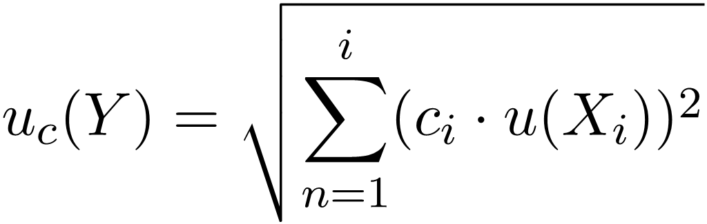
If the input variables are uncorrelated, the combined measurement uncertainty uc(Y) of a target quantity Y can be calculated from the standard uncertainties of the input quantities ui(X) as follows (Schwarz, 2020a):
 |
(2) |
wherein,
- ci – Sensitivity coefficient, defined as ci = ∂f / ∂xi
- u(xi) – Standard uncertainty of the input quantity xi
- n – Number of input quantities
The uncertainty uc is propagated from the uncertainties of the inputs using a first-order Taylor series expansion (linear approximation). The sensitivity coefficient is derived from the partial derivative of the functional model (Y=f(X)) with respect to the input quantities, which indicates the effect of each input quantity on the final results. This represents the case where functional model is linear and no correlation is assumed between the input parameters.
The concept of GUM, defines a CI around a measured value called expanded uncertainty. The true value of the measurand is expected to lie within this interval. Mathematically, it is represented as:
where k is the coverage factor, determined based on the desired Confidence Level (CL). Thus, the final measurement result can be expressed as:
2.1 Establishing the measurement model
In this case, the measurement model is the solution of the coordinates in the target coordinate system. The goal is to derive the absolute coordinates of the waterbed from the raw measurement data collected by the installed sensors. This derivation occurs in multiple steps and is relative to different reference systems.
Step 1 – Deriving coordinates within Transducer coordinate system (T-Frame): Coordinates in the T-Frame are derived based on transducer measurements (range r, beam angle θ) as follows:
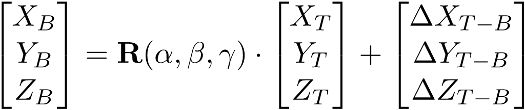
Step 2 – Transforming into Ship’s coordinate system (B-Frame): In the B-Frame, the X-axis runs along the ship’s length (positive toward the bow), and the Z-axis points toward the zenith of the ship. The Y-axis corresponds to the port side direction. The origin of this coordinate frame is the ship’s Center of Gravity (CoG). Coordinates in B-Frame are obtained by a 6DOF transformation: first, the coordinates in T-Frame are rotated based on mounting angles of the transducer with respect to the ship body frame (denoted by α, β, and γ), and then they are translated based on the coordinate difference between the transducer’s reference point and the ship’s CoG. This translations in XYZ(ΔXT-B, ΔYT-B, ΔZT-B) are determined in a vessel offset survey.
 |
(6) |
Step 3 – Transformation from B-Frame into the Local topocentric coordinate system (LL-Frame): Measurements from the Global Navigation Satellite System (GNSS) sensor are obtained in the LL-Frame, which has globally defined axes: The Y-axis points toward geographic north, and the Z-axis runs parallel to the plumb line, pointing toward the local zenith. The translation values in XYZ (ΔXB-LL, ΔYB-LL, ΔZB-LL), are based on the coordinate differences between the ship’s CoG and reference point of the GNSS antenna. Due to the axis orientation in the UTM system, αH is introduced, which results from the heading according to αH = 90° – H. The rotation is based on the measured heading αH, pitch P and roll R by Inertial Measurement Unit (IMU).
 |
(7) |
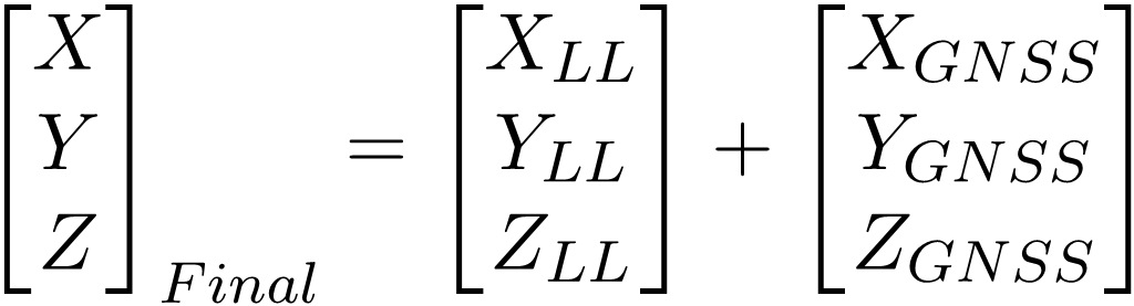
Step 4 – Combining with GNSS Measurements: The final coordinates are obtained by combining the transformed coordinates in LL-Frame with the GNSS measurements from the GNSS:
 |
(8) |
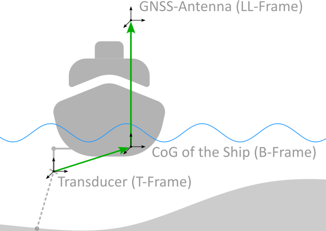
This generalized formulation describes the measurement system illustrated in Fig. 1 and applicable to different sensor types and fields of application.
2.2 Identifying influencing factors
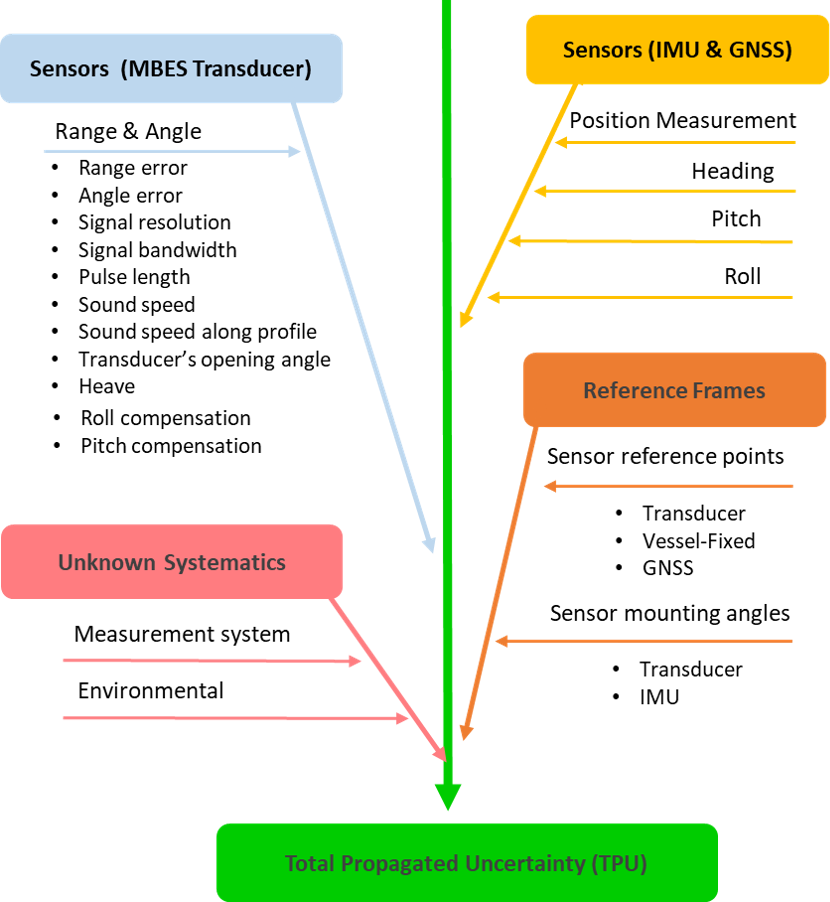
Once the measurement model has been established, the next crucial step is to identify all elements that influence the accuracy of the final quantity. These factors arise from the sensors themselves – including their quality and the reliability of the source data – environmental conditions, and the definition of the chosen reference frames. In the case of an MBES, not only must uncertainties in measured range and angle be considered, but also indirect influences such as variations in sound speed at different depths, the transducer’s opening angle, pulse length, beam bandwidth, and heave. In addition, the precise alignment of the sensors relative to one another and the careful definition of reference points play a vital role in ensuring accurate results. The main factors influencing bathymetric measurement uncertainty are illustrated in Fig. 2. For a deeper discussion of each uncertainty source, its overall impact, and the methodologies to quantify it, readers are referred to (Hare, 1995) and (Wirth, 2011).
2.3 Uncertainty estimation
With the measurement model established and the relevant influencing factors identified, the next step is to estimate the uncertainty of the target quantity via error propagation. Classical GUM propagation (refer to Eq. 2) involves computing the derivatives of the measurement model for all influencing parameters. However, because our measurement model is highly nonlinear, the classical approach is suboptimal. For complex systems, an alternative solution is to use Monte Carlo Method (MCM), as described in GUM (ISO, 1998). MCM offer several advantages: it overcomes the limitations of classical GUM propagation – which assumes small uncertainties and relies on a first-order Taylor expansion – and it accommodates any Probability Density Function (PDF) of input parameters, thereby extending the analysis beyond the constraints of normal distributions. The outcome of MCM is not just a standard uncertainty, it also gives a complete uncertainty distribution.
To estimate uncertainties using MCM, it is first necessary to identify the PDF corresponding to each influencing factor. MCM is based on performing a large number of simulated random experiments, and its validity is ensured when a sufficient number of trials are conducted. Typically, the number of samples ranges from 1,000 to 1,000,000 (e.g., m = 100,000 in Alkhatib et al. (2009) and m = 1,000,000 in Schwarz (2020b)). Due to its computational intensity, it is imperative to optimize the number of samples to achieve a balance between computational efficiency and result accuracy (ISO, 1998; Schwarz, 2020b).
The outcome of MCM is the PDF of the parameter of interest, which represents the combined measurement uncertainty. The three-dimensional expanded uncertainty, at a 95 % CL, is defined as the TPU. As specified by the IHO (2022), the TPU consists of two components: TVU and THU. The TVU is extended uncertainty in vertical dimension (σHeight). Similarly, THU is a two-dimensional uncertainty for the North and East dimensions (σNorth, σEast). For normally distributed, one and two-dimensional variables, The IHO defines an expansion factor of 1.96 and 2.45, respectively. Known systematic deviations Uc can also be incorporated. TVU is calculated as:
 |
(9) |
and THU is calculated as:
 |
(10) |
3 Validation of the uncertainty model
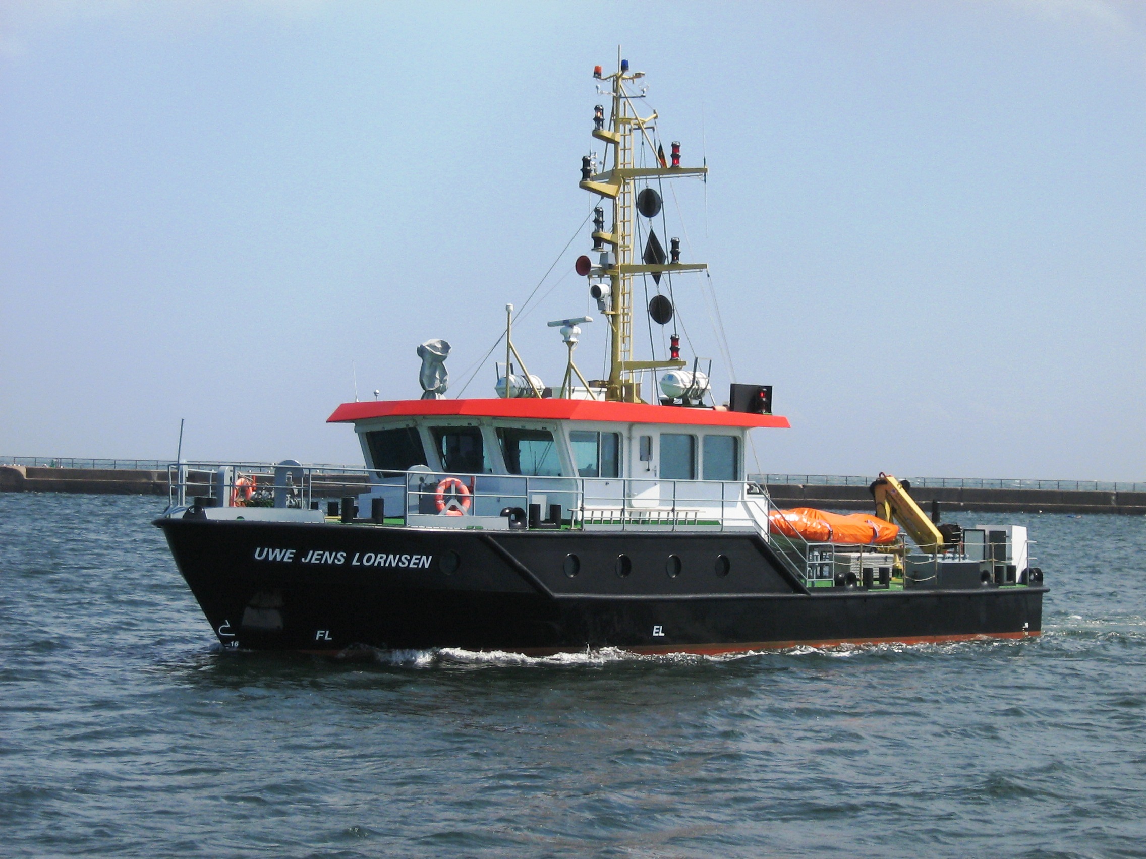
To assess the functionality of our model and validate its performance, we use real data. Although the systems and configurations of measurement instruments may vary across different vessels, their underlying principles remain similar. In this study, we focus on a specific measurement system – the Uwe Jens Lornsen (UJL; Fig. 3). We developed the measurement model for UJL according to Section 2.1, and for a specific measurement campaign, a complete uncertainty model is also established.
3.1 Details of the measurement system
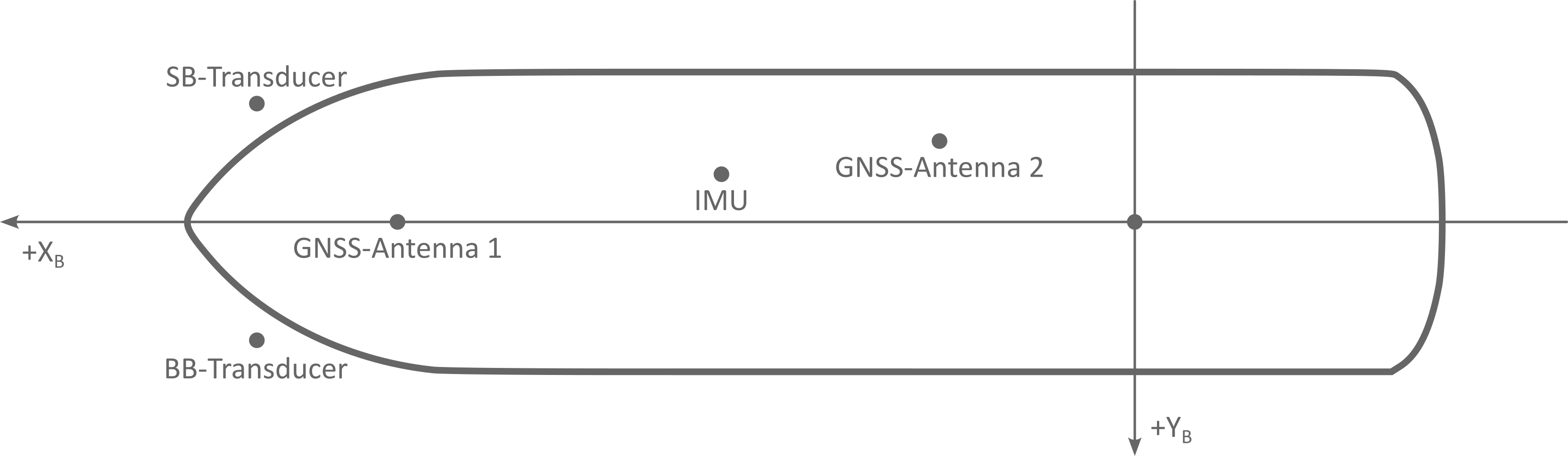
The survey vessel UJL (Fig.3) is a survey vessel operated by the Elbe-North Sea (Tönning) Waterways and Shipping Office (WSA). Built in 1993, its primary tasks include monitoring and depth surveying of maritime navigation channels along the Schleswig-Holstein West Coast to ensure safe and efficient navigation. Additionally, UJL is used for surveying structures, harbors, and dredging areas. To perform these tasks, the UJL uses a Kongsberg EM2040C dual-head multibeam echo-sounding system with two permanently installed transducers. For spatial referencing, a satellite-based positioning system – comprising PDGNSS with an integrated navigation sensor system (INS), including a Seapath 330+ and a motion reference unit (MRU 5+) – is used. The location of the sensors on UJL is shown in Fig. 4.
The primary sampling sensors used on UJL is MBES. Two MBES are mounted perpendicularly to the vessel, enabling a profile-based scanning of the seafloor. For efficient scanning, these two echo sounders are oriented along the port–Back Board side (BB) and Star Board side (STB) and tilted at 37° relative to the ship’s baseline. In addition to the dual-head system, a third hydroacoustic sensor – a Single Beam Echo Sounder (SBES) – is used to measure the central depth at the vessel’s nadir using various frequencies. Note that the SBES was used exclusively for navigation support and was not involved in the bathymetric data processing or experimental analysis.
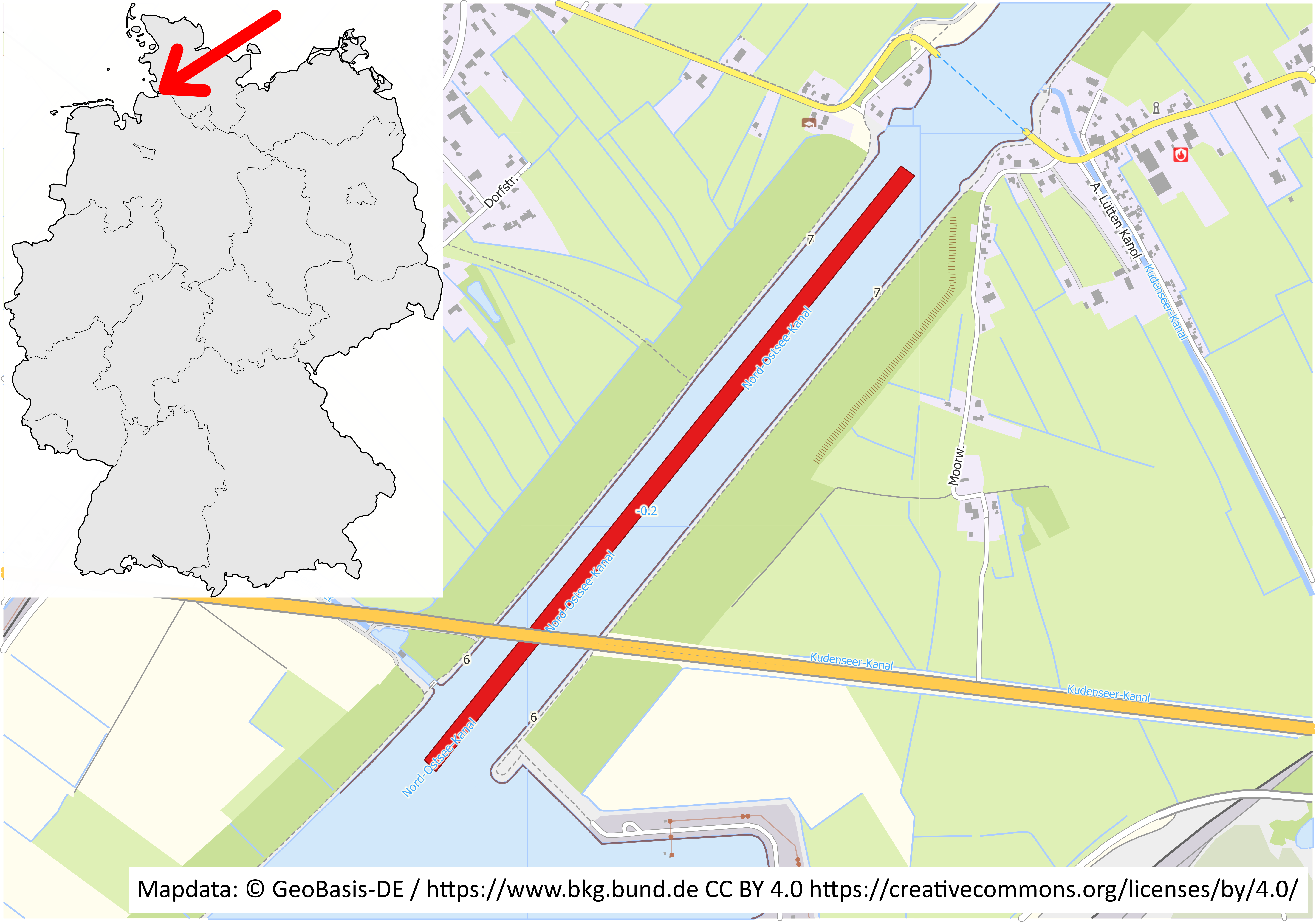
The UJL was used in 2019 for a measurement campaign of the man-made Kiel Canal (Fig. 5), conducted by the Elbe Nordsee Waterways and Shipping Office (Tönning). A 300 m long measurement swath was used as test data. In the selected section of the campaign, both flat areas and structured regions characterized by small bed load transport bodies (dunes), embankments, and leaps across flow direction were observed. The riverbed in this area typically consists of rock, silt, and gravel; water depths reach up to 13 m. The ‘equal angular’ measurement mode produces 256 measurement points per ping, with an across-track distance of around 0.06 m near nadir and 0.4 m in the remote swath areas. Near the vessel’s nadir, the point density is approximately 45 points per square meter, decreasing to 15 points per square meter in the outer regions. Based on the vessel’s speed and the chosen sampling rate, the pings have a typical along track distance of 0.35 m.
The test area exhibits varying effects on the measurement uncertainty due to the combination of high-water depth with partly shallow areas characterized by sediment and partly sloping embankments. The geometry of the observation configuration changes significantly – for example, the measured distance, the angle of incidence, and consequently, the size of the measurement footprint varies considerably. Furthermore, different structures such as small dunes or leap areas provide distinct backscattering properties, each influencing the measurement uncertainty in a unique way.
3.2 Uncertainty model for UJL
All sensors deliver the raw data in their specific sensor coordinate frame. To retrieve a 3D PC in the target reference frame, the measurements must first be transformed to a consistent vessel reference frame and then to the target reference frame. Section 2.1 outlines the methodology for calculating the seafloor coordinates for a single transducer. Following this methodology, we establish the measurement model for UJL, where the target coordinate system here is ETRS89/DREF91 (realization 2016) with UTM projection.
A detailed list of the key parameters and their corresponding uncertainty values, as incorporated into our uncertainty modeling, is presented in Table 1. For those parameters marked with “e.g.”, the listed values are representative examples from the dataset and are not treated as fixed. Instead, they are dynamically estimated per observation within the simulation, using established models such as the geometric range uncertainty model of Hare (1995) and Wirth (2011), which incorporate relevant factors like slant range, beam angle, and sound speed variability. For more details on each uncertainty source and the methods used to quantify them, readers are referred to Hare (1995) and Wirth (2011).
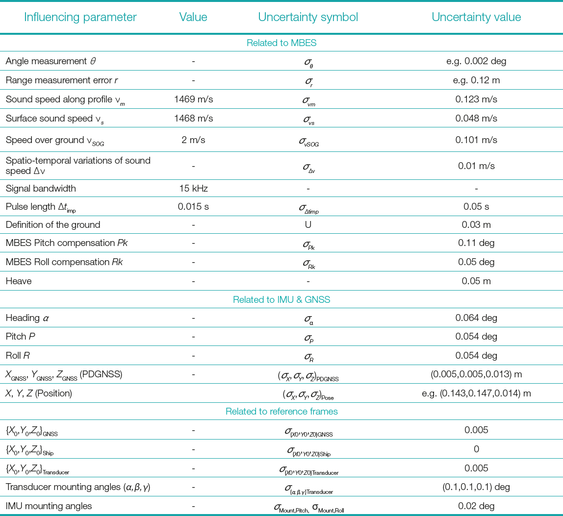
Here, we assume normal distribution for all parameters considered, as listed in Table 1. In this approach, input parameters are assumed to be statistically uncorrelated. Nevertheless, correlations that naturally arise through the functional relationships between variables are implicitly captured by the Monte Carlo Simulation process. The different variations of the input parameters propagate through the nonlinear system model, and their mutual effects on the target variables (X, Y, Z coordinates) are reflected in the output’s distribution. The uncertainties are calculated separately for each coordinate component, providing individual uncertainty values for the East, North, and Height components. Following the MCM, 1000 simulations were performed, resulting in 1000 solutions for each point and its East, North, and Height components. The PDF of one example measurement point’s coordinate solutions is illustrated in Fig. 6 as an example. A normal distribution has been estimated for each component and shown with red lines in Fig. 6. The calculated coordinates align well with the Normal distribution curve, with no significant deviations observed. Therefore, we use standard deviation corresponding to a CL of 68 % to determine uncertainties of each component (σEast, σNorth, σHeight). These uncertainties are then used to calculate TPU values (Eqs. 9 and 10).
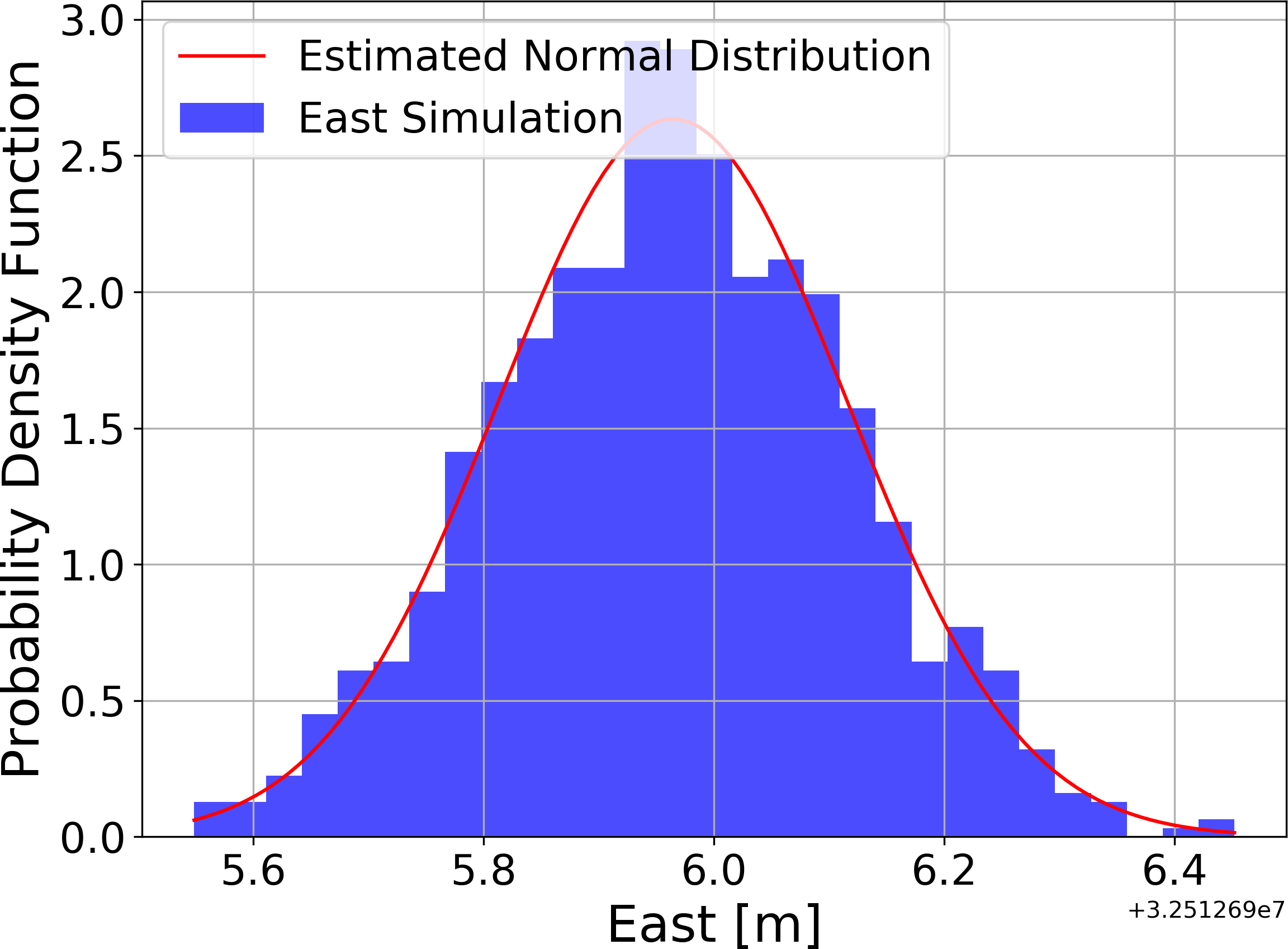
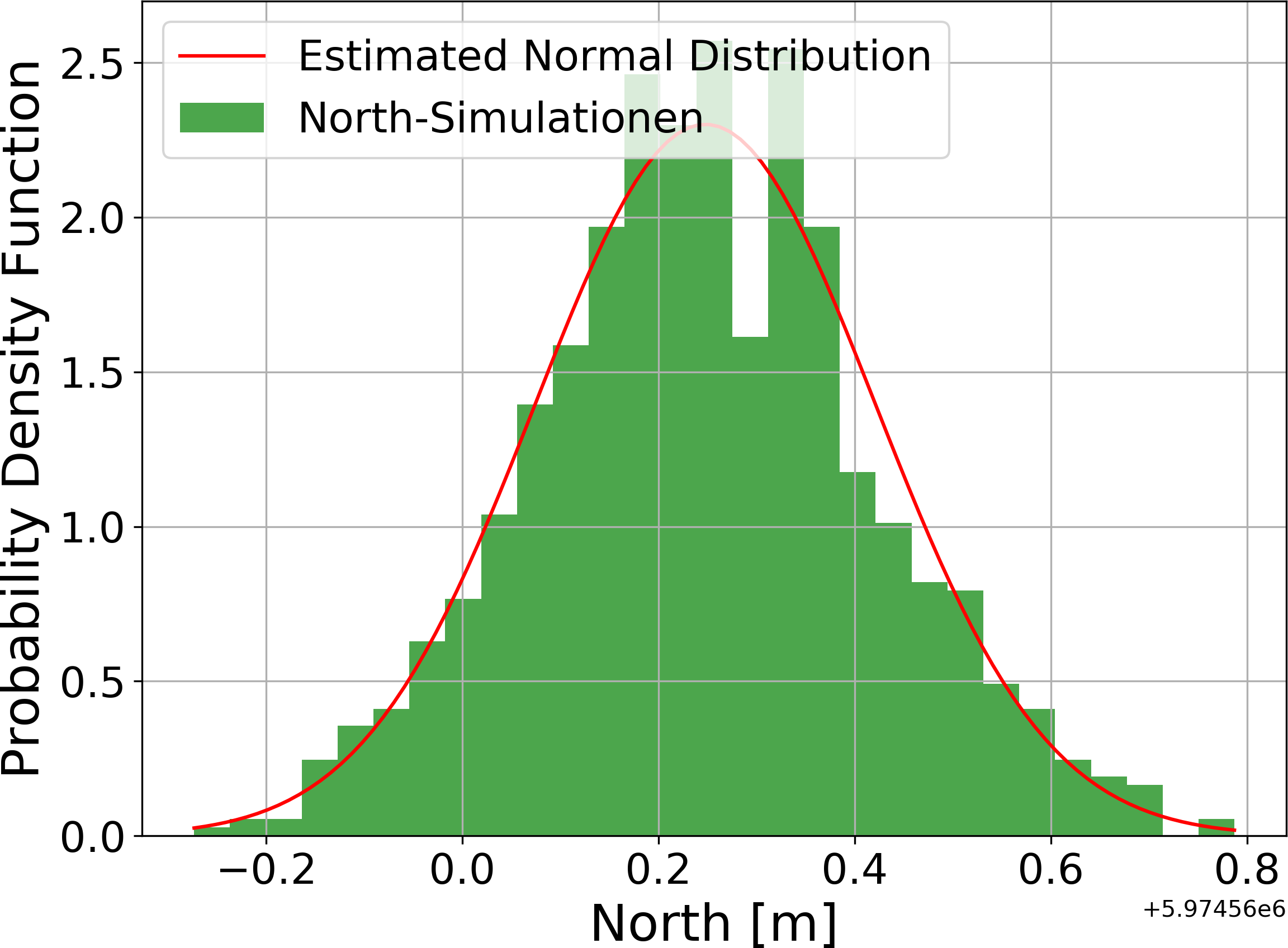
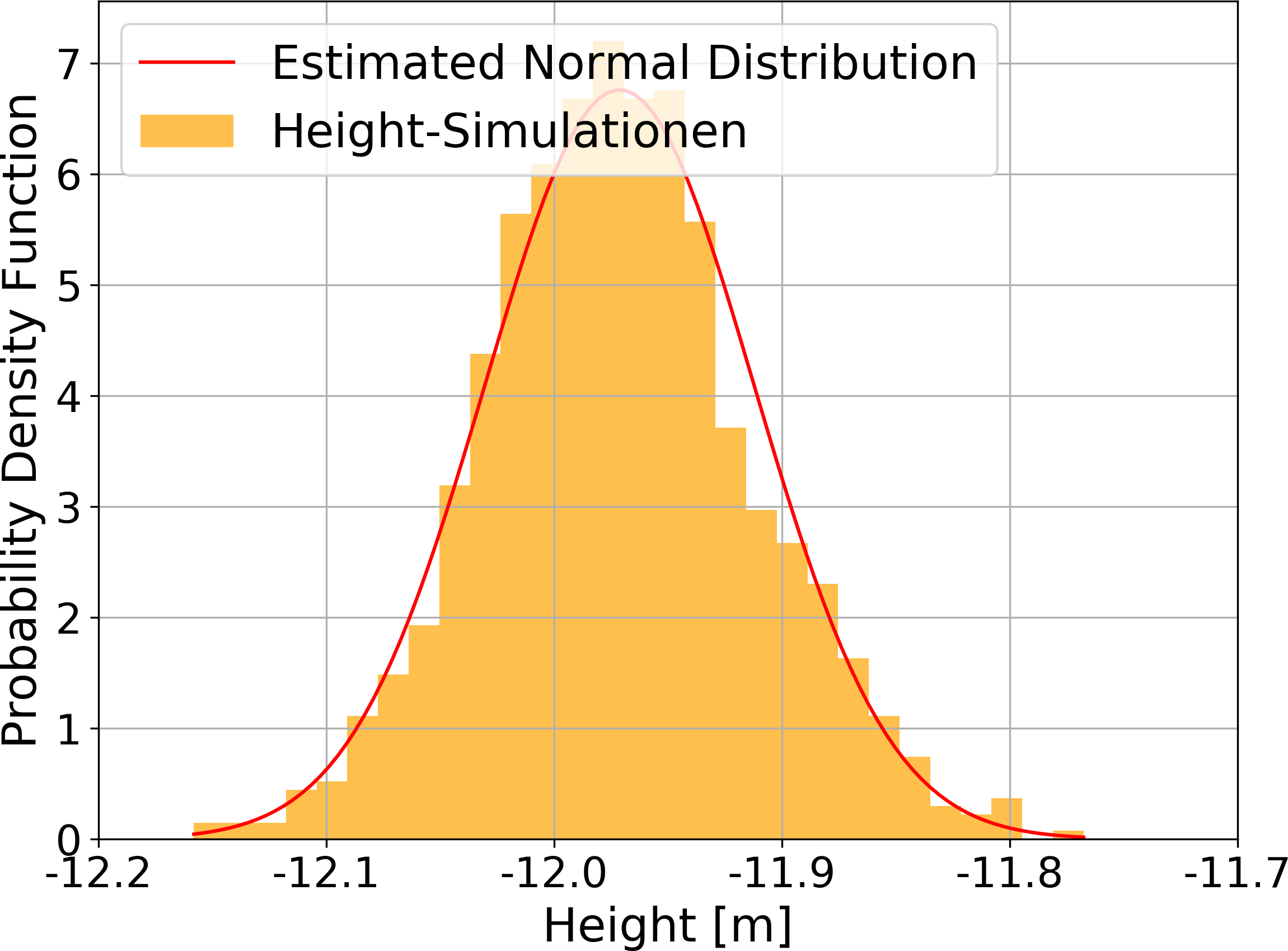
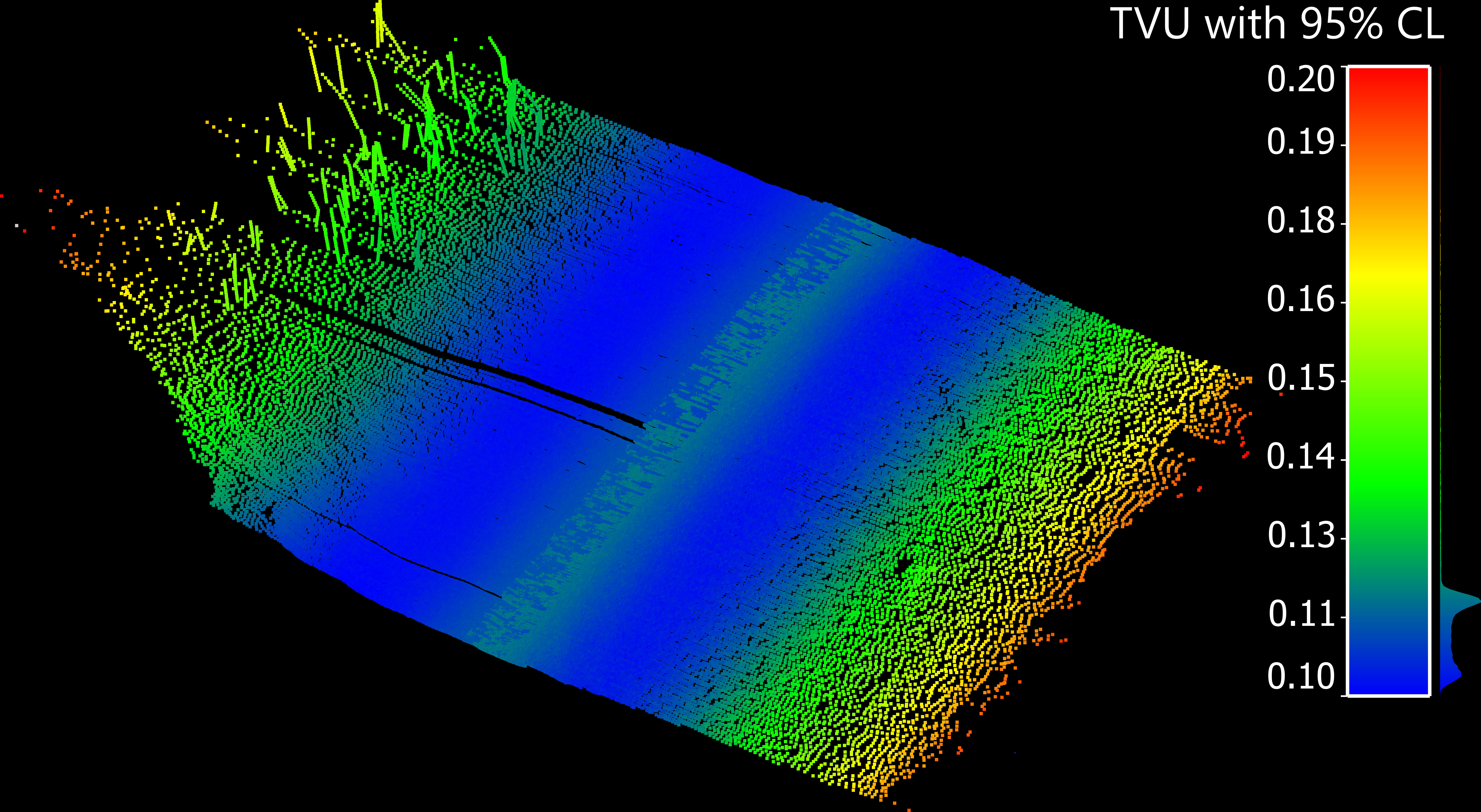
Fig. 7 illustrates the results of the MCM uncertainty calculation with 95 % CL for each measurement point. Here, uncertainties are expressed at a 95 % CL, in accordance with the definition of TPU (see Eqs. 9 and 10). The previously calculated standard uncertainties (at 68 % CL) are used as the basis for this propagation. Fig. 7a shows the height uncertainties for the first 100 profiles within the measurement swath, while Fig. 7b presents the horizontal uncertainties. These figures include measurements from both BB and STB transducers, with coordinates color coded according to their calculated TVU and THU. The color scale is provided in the legend. In the height component, uncertainties vary significantly within a single profile, ranging from 9 cm directly under the ship to 29 cm for the outer transducer beams. This variation aligns with the expectation that measurement uncertainty increases with greater measured distances and larger beam angles. Additionally, a slight increase in uncertainty is observed in the direct nadir area. This increase in TVU is mainly due to limitations in signal resolution. At nadir, where the acoustic path is shortest and perpendicular, pulse duration plays a dominant role in depth resolution. Similarly, horizontal uncertainty increases with distance from the vessel due to larger beam footprints and weaker signal returns at steeper angles. In outer swath areas, small errors in angle or range are amplified, leading to greater horizontal position uncertainty. However, the range of the horizontal uncertainty values differs considerably from that of the height uncertainties, varying from 0.55 m near the nadir to 1.28 m in the outer beams. This confirms that horizontal uncertainty is generally higher than height uncertainty.

3.3 Discussion of TPU modelling results
To validate the results of the uncertainty analysis, we compared our MCM results with those obtained using the classical GUM approach and those estimates from the commercial software QINSy (version 8.18.3; QPS, 2025), which is used as the data acquisition software on UJL. In this software, the offsets in the vessel frame and the measurement data from the sensors are converted into a 3D PC as projected points in the official reference frame. In addition, other attributes recorded by the sensors are included so that a TPU value per beam can also be determined and specified. The exact procedure for determining the TPU by QINSy is not known, but tests and comparisons suggest that the procedure is similar to the methods described in (Hare, 1995; Wirth, 2011). Nonetheless, it is presumed that QINSy’s TPU estimations meet hydrographic standards and provides combined standard uncertainties with 95 % CL.
According to IHO, each survey must comply with a defined “maximum allowable uncertainty” for both vertical and horizontal measurements. For vertical uncertainties, permissible limits at a 95 % CL are computed based on depth-dependent b and depth-independent a parameters, as well as the actual depth d (Eq. 11). These parameters differ according to the survey order as described in IHO (2022). Furthermore, the S-44 standard defines maximum permissible horizontal uncertainties; for example, the maximum horizontal uncertainty THUmax allowed for Special Order surveys is set to 2 m
(IHO, 2022).
 |
(11) |
Fig. 8 presents the TVU of measurement points for a single representative profile to illustrate the structure and variation of the uncertainty with respect to beam angle relative to the ship’s vertical axis (Fig. 8a) and lateral distance (Fig. 8b). While this profile is not intended to be statistically representative of the full dataset, it provides a clear example of the underlying trend. The plots compare solutions from the classical GUM approach, MCM, and QINSy. The uncertainties for BB and STB transducers are shown with similar color. Fig. 8 additionally illustrates the maximum permissible vertical uncertainty TVUmax for the Special Order and Exclusive Order survey as defined by the IHO (2022), for a mean depth of 12 m. The uncertainties computed via MCM follow the expected pattern shown in Fig. 7a. As shown in Fig. 8a, TVU increases exponentially with respect to the beam angle, while Fig. 8b shows a more linear increase in TVU with lateral distance from the vessel. The lowest uncertainties occur at distances of 12–15 m from the ship, corresponding to beam angles of 48–53° from the ship’s normal. This effect is primarily attributed to limitations in vertical resolution caused by pulse duration. The nadir beams, pointing directly downward, rely almost exclusively on the two-way travel time of the acoustic pulse to determine depth. Consequently, any uncertainty in echo detection, especially when longer pulse durations are used, directly translates into vertical measurement uncertainty. While side beams are more affected by geometric distortion due to effects such as decreasing signal intensity and increasing footprint resulting from beam divergence, nadir measurements are more sensitive to temporal resolution. Additionally, the nadir represents a transition zone between the BB and STB swaths. Here, overlapping beams from both swath edges – where positional and angular uncertainties are typically higher – may interact, compounding the overall uncertainty in this central region. While all three solutions exhibit similar trends, differences exist. The classical GUM approach does not capture the nadir effect seen in MCM results. Since both methods are based on measurement model described by Wirth (2011), only minor discrepancies are expected. These variations likely stem from differences in user-defined input parameters, highlighting their role in uncertainty analysis. Compared to QINSy’s uncertainties, the relative variation aligns, but our uncertainty model appears to account for similar factors with differing absolute impacts. All three predicted uncertainties are below TVUmax for the Special Order survey. In Fig. 8, we observe that the outer-beam uncertainty of the BB transducer exceeds the Exclusive Order threshold defined by the IHO S-44 standard. According to S-44 standards, the TVU is expected to increase with water depth, following a depth-dependent model (IHO, 2022). However, the measurement campaign analyzed in this study was conducted in a relatively uniform depth environment, with an average depth of approximately 13 meters. As a result, the data do not capture a wide range of depth-induced variability in TVU. Future work in more bathymetrically diverse areas may provide further insight into this relationship.
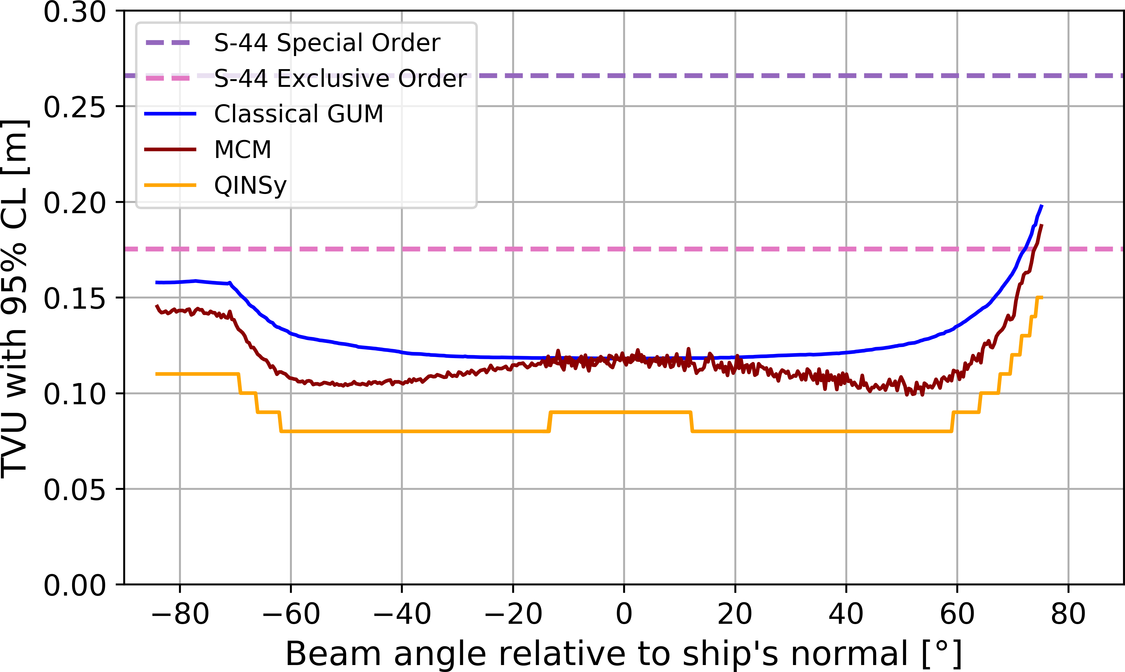

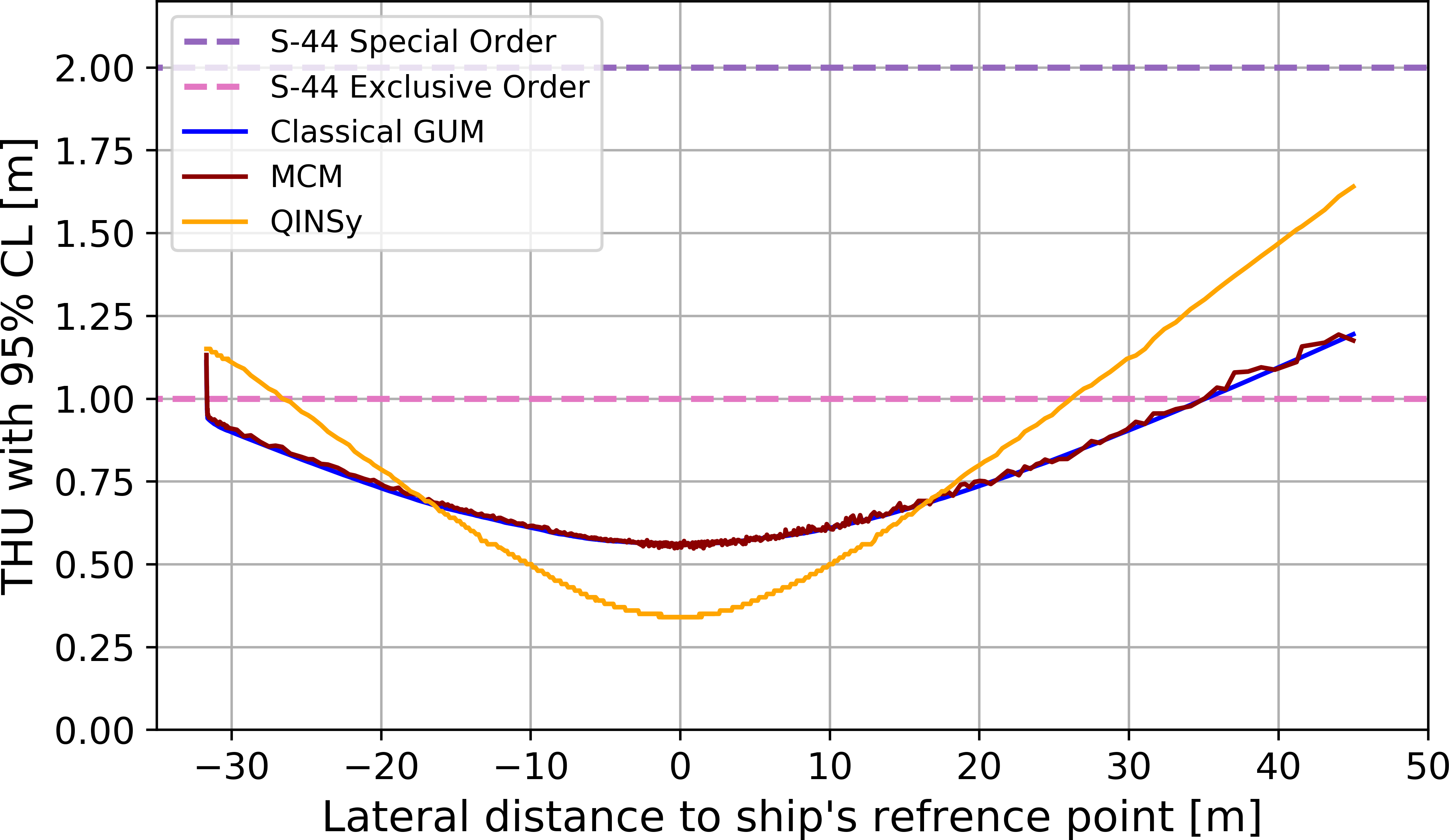
Fig. 9 presents estimated THU for the same profile measurement. It compares the results from MCM, GUM, and QINSy’s THU values. The uncertainties for BB and STB transducers are shown with similar color. Fig. 9 also shows the maximum permissible horizontal uncertainty THUmax for the Special Order survey as defined by the IHO (2022), represented by the dotted line.
Compared to height uncertainty, horizontal uncertainty is substantially higher. The uncertainty profile also differs, showing no increased uncertainty in the nadir. The comparison across methods reveals minimal differences between GUM and MCM results. To highlight this, Fig. 9b provides a close-up of the nadir region’s uncertainty results. The MCM solution is noisier due to its reliance on simulation rather than linearization, as with the classical GUM method. Larger deviations appear in comparison with the QINSy solution. Particularly in this profile, in the nadir region, QINSy’s uncertainty values are roughly 20 cm lower than those from GUM and MCM. Conversely, QINSy’s uncertainty increases more significantly in the outer beams. In average the difference between our uncertainty model (both realizations MCM and GUM) and QINSy, along the profiles and for all the 3000 measured profiles, is around 17 cm. This suggests that positional uncertainty influences are modeled differently across methods, and further investigation into QINSy’s calculation approach would be required to fully understand these discrepancies. All three predicted uncertainties remain below the THUmax threshold defined for Special Order surveys; however, at the swath boundaries, they exceed the stricter 1-meter limit specified for the Exclusive Order.

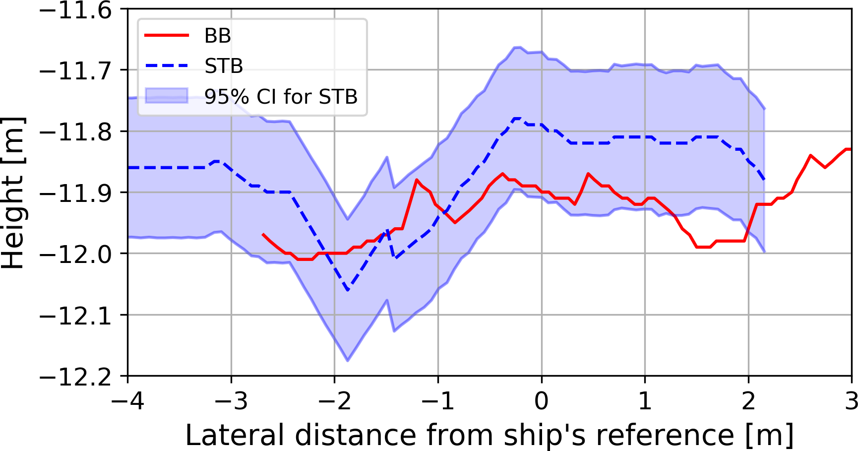
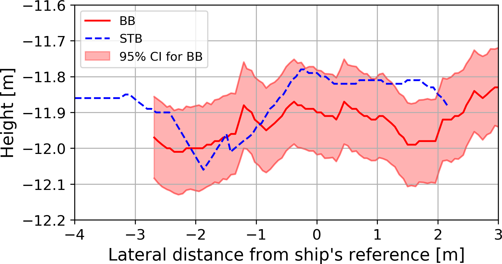
This research primarily focuses on un)certainty solutions derived from MCM. To assess the plausibility of the estimated TPU values, we analyze the overlap area where the BB and STB transducers record measurements simultaneously. This region offers a valuable opportunity to validate the model’s accuracy. The two independent transducers measure the same physical surface in this region under slightly different conditions. Since the modeled uncertainty is expressed at the 95 % CI, we expect that, statistically, approximately 95 % of the measurements from one transducer should fall within the confidence interval predicted by the model using the measurements from the other transducer. Moreover, although the two transducers are internally similar, they are physically separate sensors with independent mounting setups. Small differences in mounting geometry, alignment, and calibration introduce slight variations between their measurements. This diversity further strengthens the validation, as it ensures that the comparison is not perfectly redundant but reflects realistic measurement variability. Fig. 10 presents the overlap area beneath the ship for one profile to evaluate height measurement uncertainty. The uncertainty, estimated using the MCM, is expressed as CI around the absolute height measurements. Fig. 10 demonstrates that a majority of the measurements from each transducer fall within the CI of the other. In Fig. 10a, 87.69 % of the BB transducer’s readings align with the confidence bounds of the STB transducer, while in Fig. 10b, 87.48 % of the STB transducer’s measurements fall within the BB transducer’s CI. Although these percentages do not reach the expected 95 % threshold, they suggest that the overlap area is well-represented by repeated measurements. In just this one presented example, the sample size in the overlap region may not be sufficient to make definitive claims regarding the 95 % CL. We observed similar coverage for other profiles as well. Moreover, as the both transducers operate independently, their different setups could influence their measurements. Despite these factors, the observed overlap percentages provide reasonable validation of the estimated CIs.
The overlap area is also analyzed to assess position uncertainty. Since position uncertainty results from a quadratic combination of uncertainties in the East and North components, it is represented as a two-dimensional confidence region. Consequently, each measured point’s uncertainty is expressed as a confidence ellipse. Fig. 11 illustrates the overlap area for position measurements, highlighting the confidence ellipses for points recorded by the BB. The semi-major and semi-minor axes correspond to East and North uncertainties, respectively, with no assumed correlation. As depicted, all STB transducer measurements fall within the BB transducer’s confidence ellipses. Unlike the height component, the 2D position measurements achieve a full 100 % overlap within their respective confidence ellipses. This result reinforces the reliability of the position uncertainty estimates obtained through MCM.
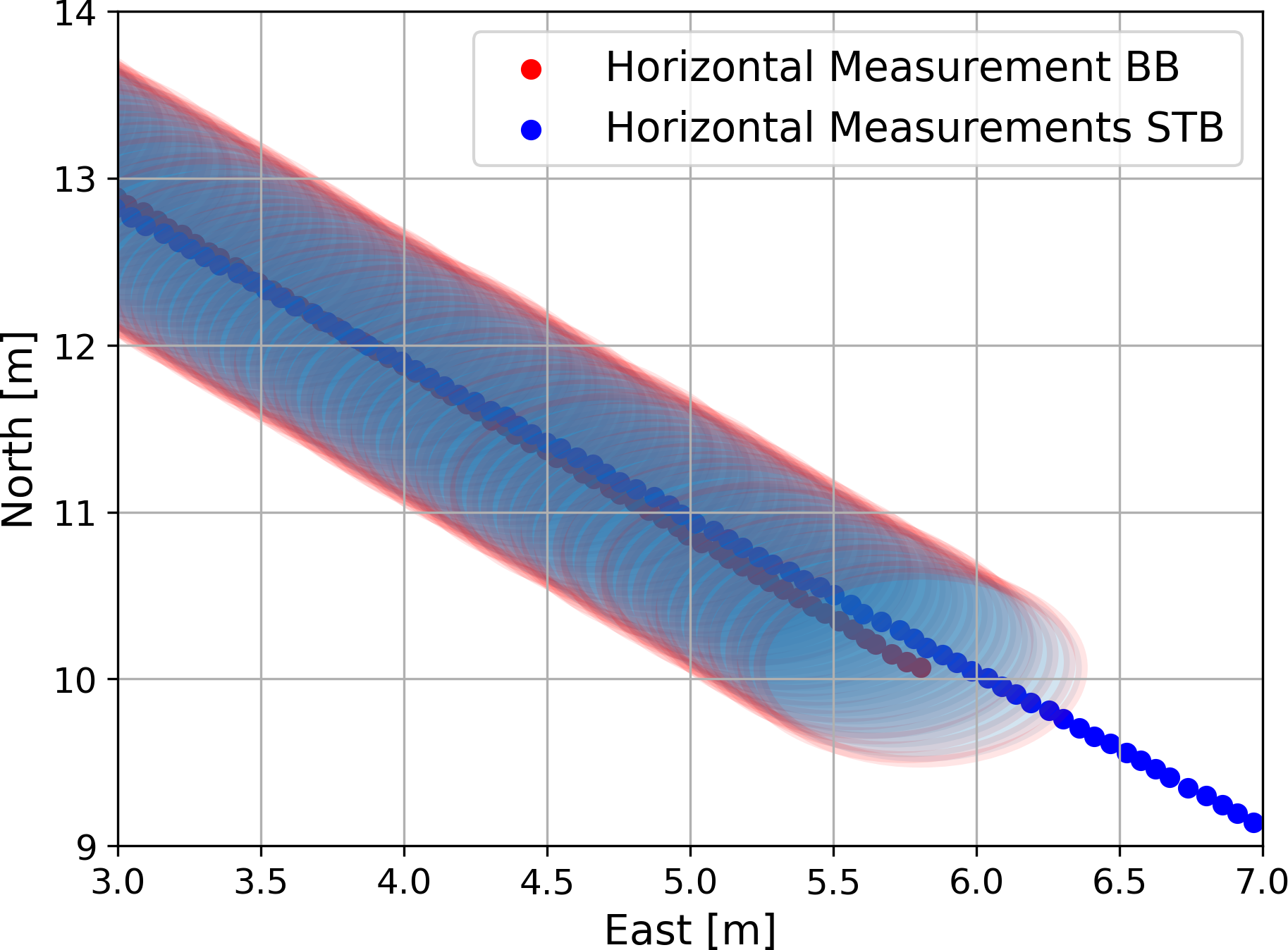
Fig. 11 Measured horizontal coordinates by STB and BB transducers with their corresponding confidence ellipses of overlapping measurement area beneath the ship. East and North are reduced for visualization.
It should be noted that there is no definitive ground truth for either the underwater geometry or the measurement uncertainty. Overall, the overlap analysis supports the validity of the developed uncertainty model. Comparisons with alternative methods further strengthen confidence in the reliability of the estimated TPU values. While systematic differences exist between models, their overall patterns remain consistent. Despite the observed systematic differences between uncertainty model and the commercial software, these deviations do not diminish the usefulness of our results. Since the primary goal of this analysis is to derive weights for the subsequent modeling step, the absolute magnitude of uncertainty is less critical than its relative distribution. The derived uncertainty values are used to construct normalized weights, directly informing the modeling process. Thus, these systematic variations will not negatively influence the outcomes in the second part of this paper. The weighting approach ensures that the subsequent analyses remain robust, as differences in the absolute uncertainty levels do not significantly affect our conclusions or the modeling accuracy presented in the later sections.
A potential empirical approach to characterizing measurement uncertainty in MBES systems would be to perform repeated high-density surveys over a flat and stable area, followed by the generation of a high-resolution averaged gridded surface. Deviations of individual measurements from this reference surface could then be used to estimate the distribution of random errors. Although not explored in the present study, such methods may provide valuable validation or calibration data for future uncertainty modeling.
A key approach to further evaluating this model is through simulation. In the next steps, we use the developed uncertainty model to simulate the ground truth, measurement process, and their corresponding uncertainties, assessing its applicability and reliability.
4 Survey simulator
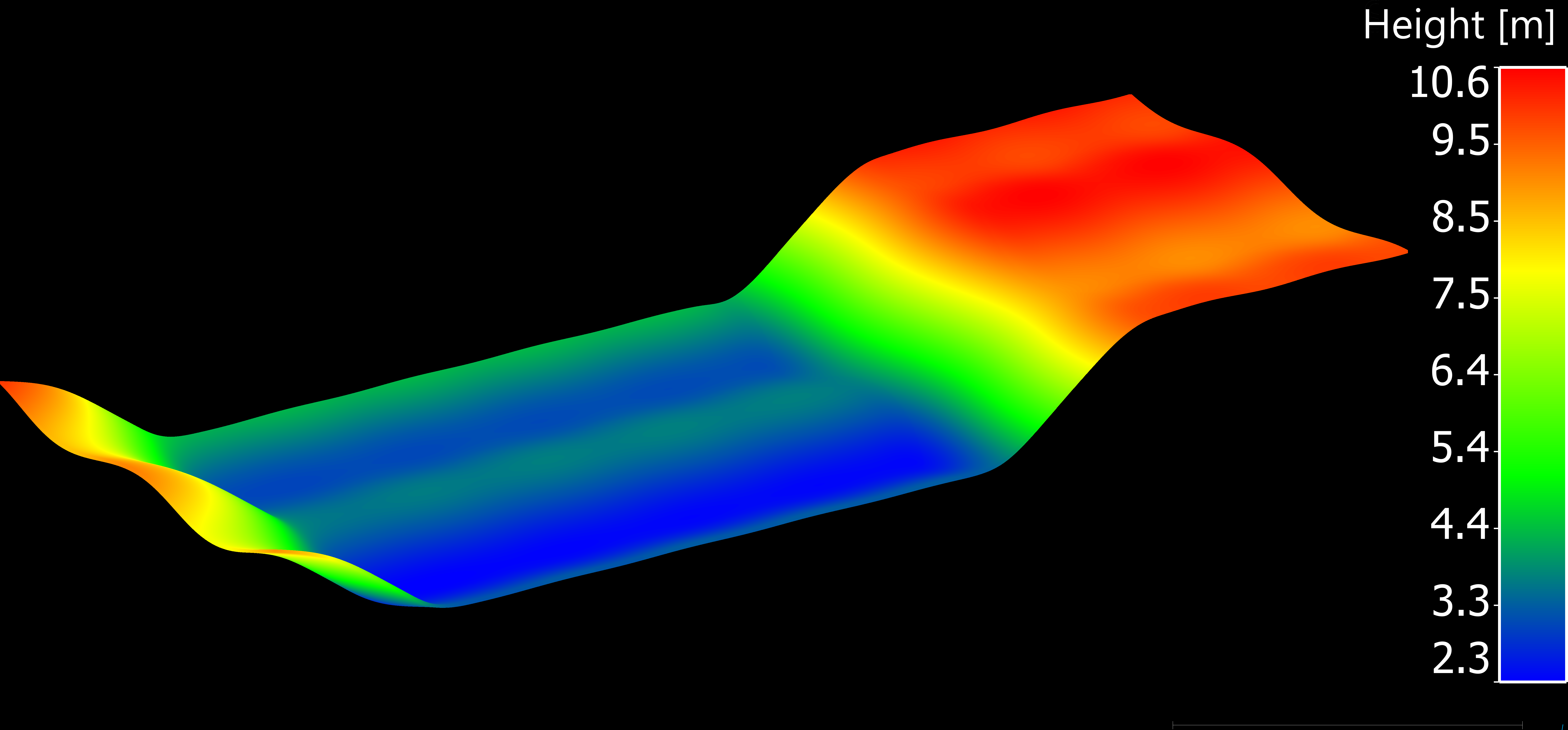
A major drawback in estimating uncertainties for bathymetric measurements is the unknown geometry of the waterbed. A synthetic dataset is used in this study to overcome this issue. The main idea is to employ a mathematically defined surface to simulate realistic bathymetric measurements. The ground truth surface is defined based on MBA approach by Lee et al. (1997). Our MBA surface is constructed using a set of predefined hierarchical B-Spline functions and is exported as a 3D-PC with equidistant point spacing of 1 cm (Fig. 12).
The simulation environment is implemented in Python using standard libraries like NumPy (Harris et al., 2020) and PyVista (Sullivan & Kaszynski, 2019). Four steps are required to generate a realistic simulated 3D-PC of a waterbed:
- Transform the generated 3D-PC into a mesh using Delaunay triangulation (Delaunay, 1934).
- Compute Cartesian coordinates by intersecting the beams of the echo sounder with the mesh of the waterbed using ray-tracing.
- Calculate the range and beam angle between the sensor and intersected coordinates on the seabed.
- Predict realistic uncertainties for the obtained coordinates by forward modeling based on the uncertainty model developed in Section 3, using the parameters described in Table 1.
After creating the original 3D point cloud with a resolution of approximately 1 cm, a Delaunay triangulation mesh with the same resolution (1 cm) was generated. The next step is to compute the coordinates of the simulated measurements on the waterbed. The measurement beams are generated according to the chosen sensor, with equidistant angular steps in the field of view of 120°, and the central beam is directed vertically downward. The environment is assumed to be uniform, and no refraction of the acoustic wave is considered, as is generally valid in shallow water areas. Therefore, each ray is treated as a straight line starting from the transducer in the direction of the beam. The intersection of the beam with the seabed surface is determined using ray-tracing; in cases of multiple intersections, the closest one is selected.
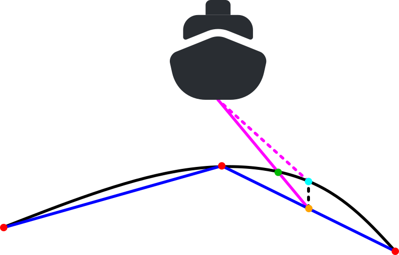
One drawback of using a triangulated mesh for the simulation is the occurrence of triangulation error, which is the difference between the generated ground truth surface and the meshed grid used for beam intersection. This error is intrinsic to the process of converting a smooth, continuous surface (the “ground truth”) into a mesh made up of flat, polygonal facets. The error is most pronounced in regions with significant curvature, as the exported points in the triangulation are connected by planar triangles.
The magnitude of this error is influenced by several factors, including the curvature of the original surface, the density of the mesh, and the quality and arrangement of the triangles. In areas with high curvature, flat triangles struggle to capture the intricate details of the surface, resulting in larger errors. While the error can be mitigated by reducing point spacing (thereby increasing mesh density), this approach increases computational cost and memory usage. While the error can be mitigated, it remains present and must be considered in the analysis. The error in Z-direction was eliminated by recalculating the Z value at the determined XY location using the original B-Spline functions, ensuring that the simulated coordinates exactly follow the surface. The reprojection process eliminates XY triangulation errors by fixing the original X and Y coordinates and recomputing the Z value based on the true B-spline surface. Thus, only the Z-coordinate is corrected, and no residual XY positional error remains after reprojection. In addressing triangulation errors, recalculating the mesh coordinates using original surface functions, like B-Splines, offers a powerful method to enhance accuracy. This technique specifically targets errors in one or more dimensions by leveraging the precise mathematical representation of the surface from which the mesh is derived. Subsequently, the range and beam angles are recalculated using the sensor’s position, and uncertainties are then predicted. The triangulation error and the projection principle are illustrated in Fig. 13.
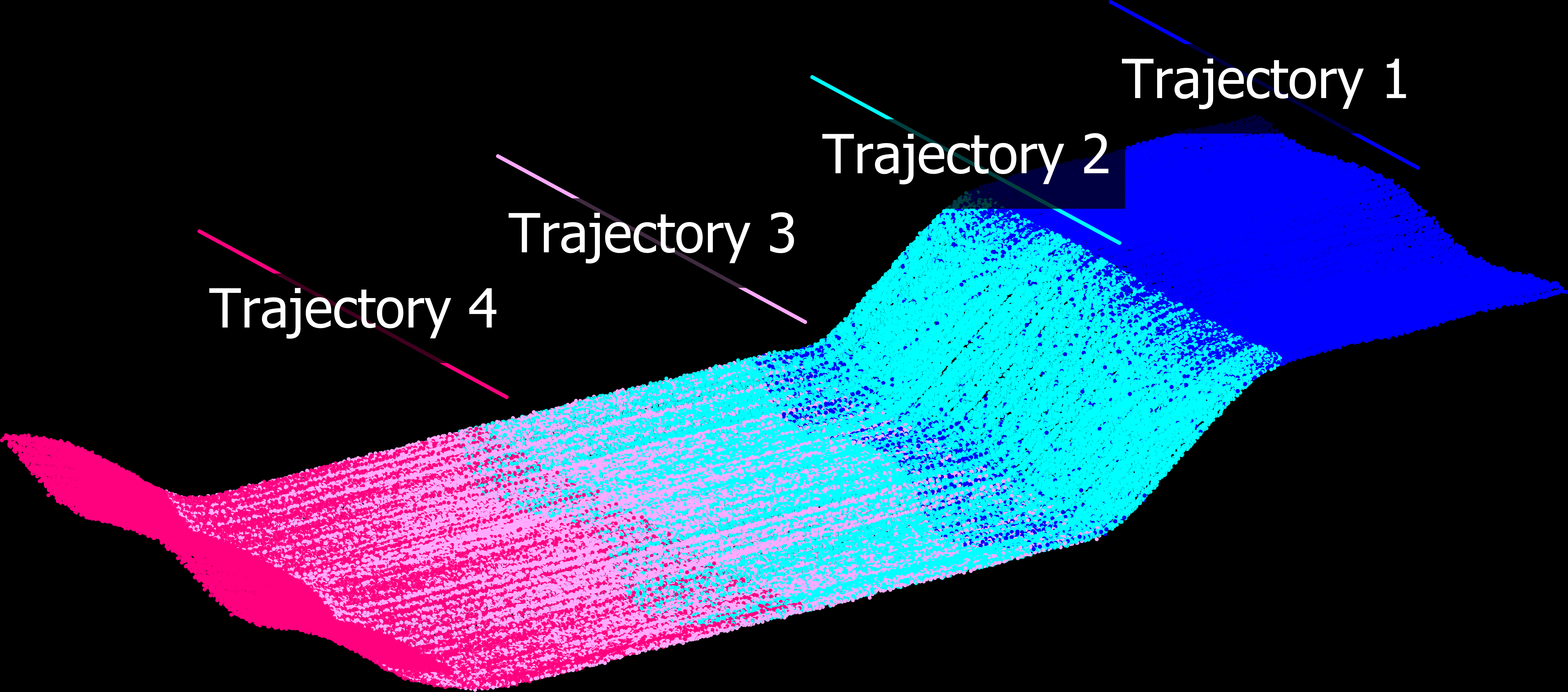
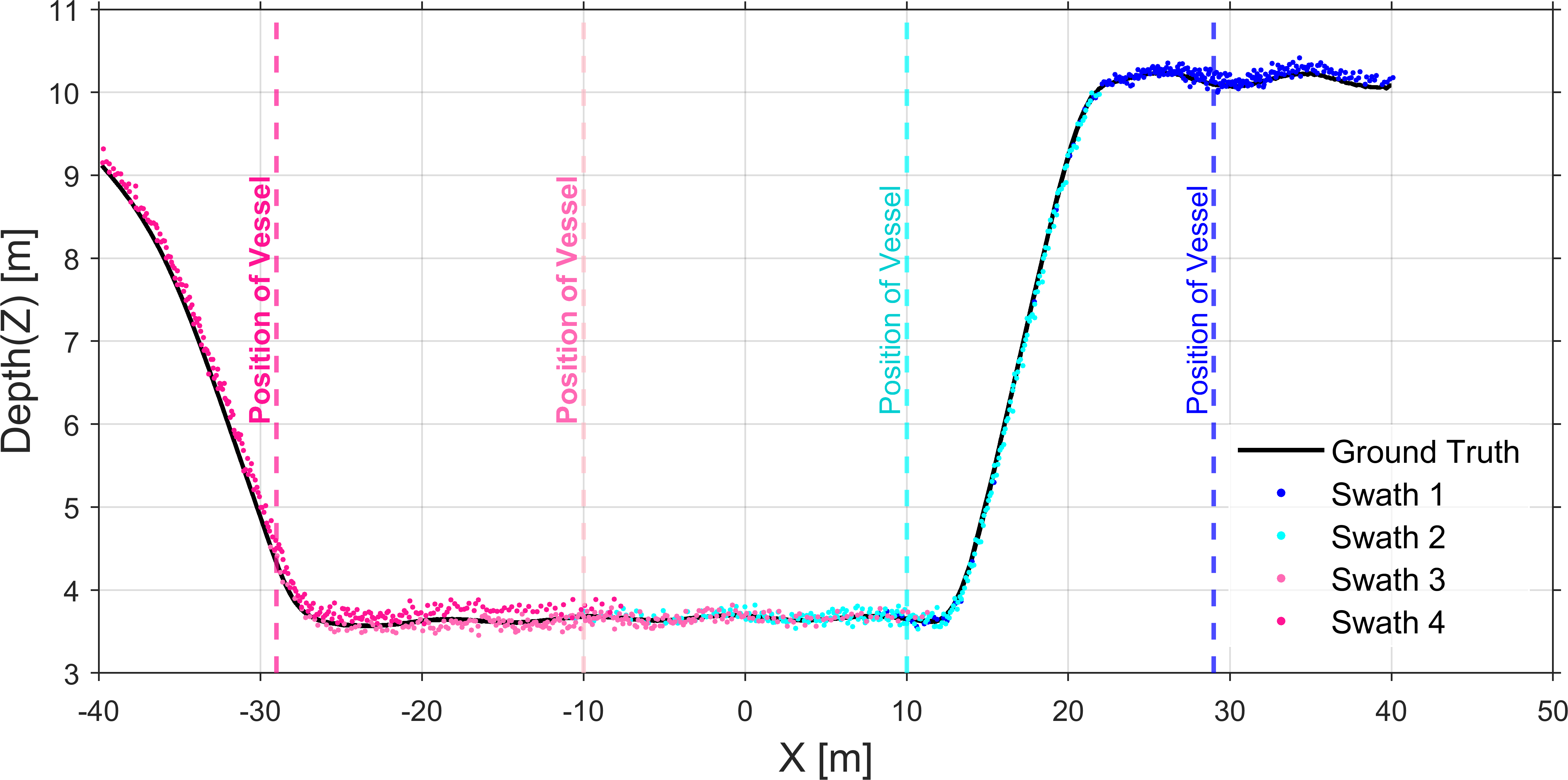
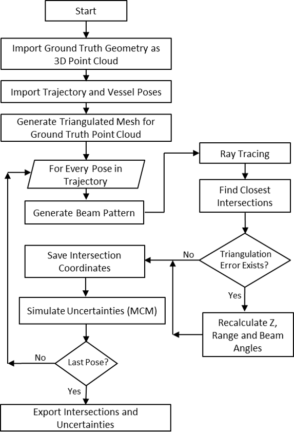
For the simulation in this study, a surface with dimensions of 80 m by 20 m and a total variation in Z-direction of 8 m is used. Four parallel trajectories are simulated to capture the entire area and to generate overlapping regions. The trajectories have an average height above the surface of 12 m above the surface and are spaced 20 m apart. The simulated surface and trajectories are shown in Fig. 14. A profile view of a random realization of the simulated measurements is shown in Fig. 15. The overall workflow of the algorithm is presented in Fig. 16.
After intersecting the beam pattern at every sensor position with the surface and recalculating the Z-value, the resulting beam angle and range readings are error-free. Realistic uncertainties are then added using the parameters and methods described in Section 3. This is performed within a Monte-Carlo simulation loop with 1,000 iterations, yielding 1,000 individual realizations for every simulated measurement. This approach facilitates a detailed analysis of the uncertainty budget, the distribution of the uncertainties, and the identification of specific ways to enhance model accuracy and reliability.
5 Measurement uncertainty and DBM
Our goal in this research is to explore how uncertainty information can be used to improve DBMs. To achieve this, we developed a simulation environment in which a known geometry is created using a precise mathematical model representing a theoretical seabed. Within this controlled environment, we simulate the measurement process while incorporating our developed uncertainty model. This setup allows us to obtain measurements that include uncertainties while retaining complete knowledge of the geometry, thereby enabling a detailed analysis of the impact of uncertainty on the final DBM.
The core idea is to integrate the estimated uncertainty information into the modeling process. For this purpose, we first clarify the type of surface model we are focusing on.
5.1 Surface model
Considering the potential complexity of underwater geometry and the characteristics of MBES data – such as high resolution, large volumes, and potential gaps – we require a method that efficiently handles these challenges while minimizing computational complexity. To achieve this, we represent the surface as a 2.5-dimensional (2.5D) model, expressed as:
 |
(12) |
where (x0, y0, z0) represents a point on the surface. To model this surface, we adapt MBA by Lee et al. (1997). The MBA method is based on hierarchical tensor product B-spline surfaces. Any point on the surface is a linear combination of control points and cubic basis functions. The B-Spline surface is defined by a grid of control points, denoted as Φ, which lies parallel to the XY-plane. The positions of these control points are predefined on the grid, serving as the basis for constructing the surface representation. To approximate the surface f(x,y), it is necessary to determine the unknown elements of Φ. This problem is structured as a linear Gauß-Markov Model (GMM), as expressed in Eq. 13 Mohammadivojdan et al. (2024). In this formulation, z represents the observation vector, while v denotes the residual vector. The matrix A is a full-rank design matrix, and Φ is the vector of unknown parameters.
 |
(13) |
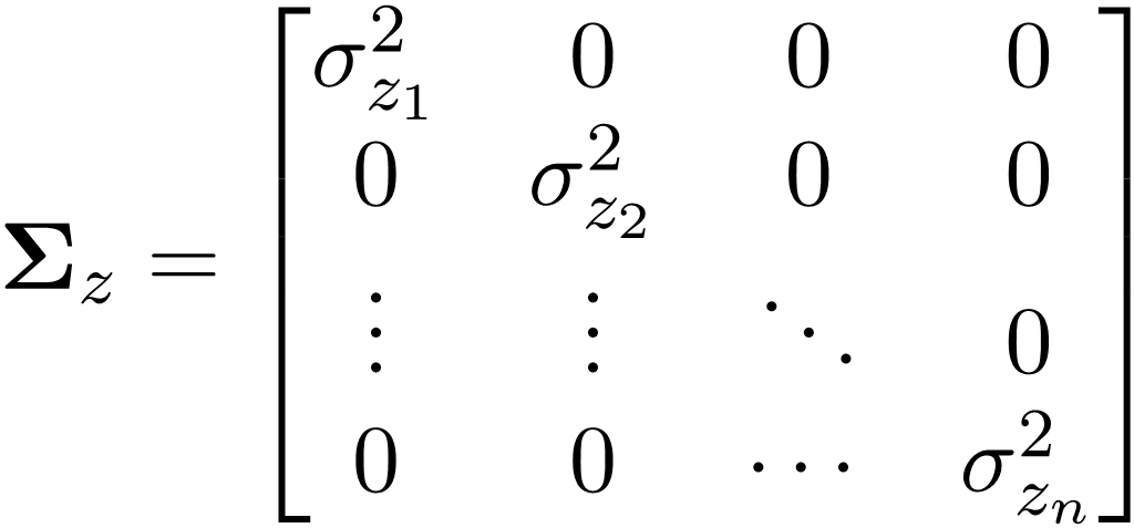
The Φ can be estimated by minimizing the sum of the squared residuals, according to Eq. 14. If the assumption is that the observations are equally weighted and uncorrelated, the weight matrix P will be an identity matrix. If information about the uncertainty of the observations is available, this P is derived as the inverse of the Variance-Covariance Matrix Σ of the observations, allowing the model to account for varying observation uncertainties. In Eq. 15, Σz represents the Variance-Covariance Matrix of the observations, structured as follows:
|
(14) |
 |
(15) |
The assumption that observations remain uncorrelated is still maintained. Incorporating the weight matrix in this way enhances the robustness of the parameter estimation, ensuring a more reliable solution while accounting for observational uncertainties.
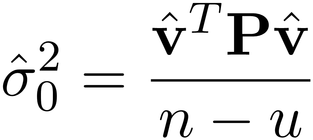
It should be noted that GMM does not directly estimate a posteriori variance factor 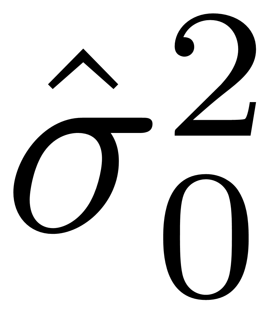 (cf. Benning, 2011, p. 144). Therefore, for evaluating the adjustment, is estimated based on
 the updated residuals v̂ as follows:
 |
(16) |
 |
(17) |
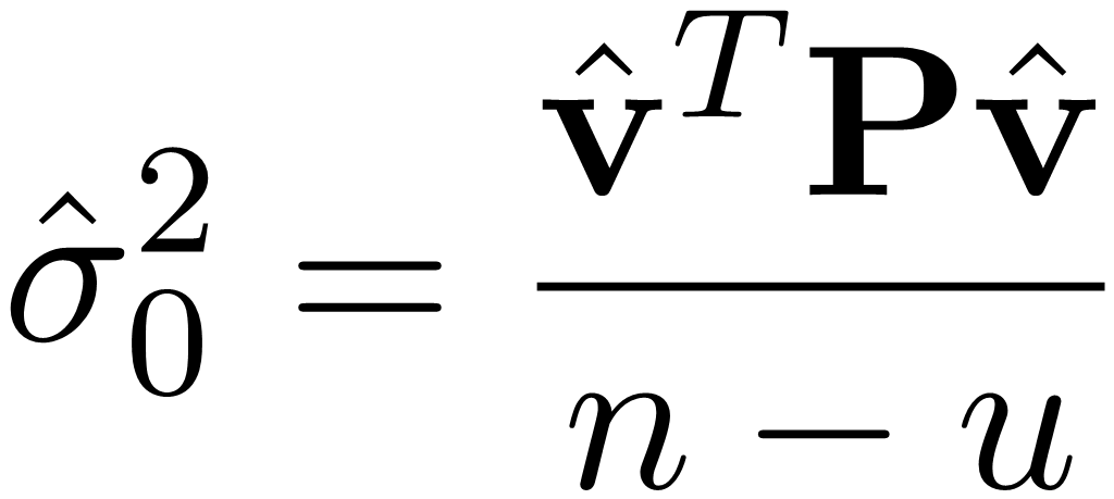
where n is the number of observations and u is the number of unknowns.
5.2 Monte-Carlo simulation experiment
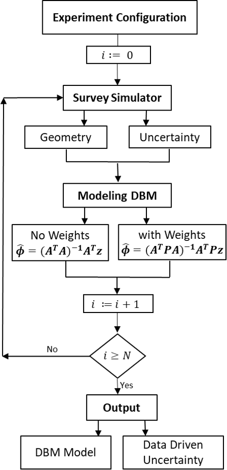
To assess the impact of incorporating uncertainties in the model estimation process, we utilize our survey simulator (see Section 4). However, a single simulation scenario is insufficient for drawing reliable conclusions; therefore, we conduct a Monte-Carlo simulation experiment, in which the entire process is repeated multiple times. By analyzing a large number of iterations, we derive more robust inferences and assessments.
In each iteration, both the geometry and the associated uncertainties are simulated and the data are modeled using MBA. Two versions of the model are generated: one that integrates uncertainty information into the estimation process and another that does not. This comparative approach allows us to assess the effect of incorporating uncertainty on model accuracy and reliability. After numerous repetitions, we determine the optimal model and extract additional insights, such as CIs or uncertainty maps, providing a clearer understanding of the model’s precision. Fig. 17 illustrates the general algorithm for the adopted Monte-Carlo simulation experiment. In this algorithm, N represents the number of Monte-Carlo iterations, which is set to 1,000 in our study.
5.3 Results and discussion
In the initial step, the focus is on evaluating model quality and associated errors in an ideal scenario assuming no measurement error is present. Although the ground-truth geometry described in Section 4 was generated using MBA functions, and the simulated data were also modeled with an MBA approach, the resulting model does not exhibit zero error. Even in the absence of simulated measurement noise, the estimated surface retains some inaccuracy. This is because the ground-truth surface was generated using a multi-layered MBA construction to introduce local deviations, while the subsequent surface approximation used a selected model complexity without reverse-engineering the original structure. Therefore, a residual modeling error naturally remains even in the absence of simulated measurement noise. This effect is expected and is analogous to real-world modeling situations where the true surface structure is unknown. These inaccuracies can arise in the simulation step or the modeling step; the simulated point cloud inherently exhibits variations in point density and spatial distribution due to survey parameters, including sensor specifications, water depth, vessel speed, measurement angles, and the underlying geometry of the waterbed. Consequently, these factors result in a non-uniform distribution of data points, inevitably affecting the final model. Additionally, selecting an appropriate model complexity is critical; an excessive number of control points might lead to overfitting, especially if the dataset includes noise or outliers. Thus, choosing the optimal model complexity requires carefully balancing smoothness against accuracy.
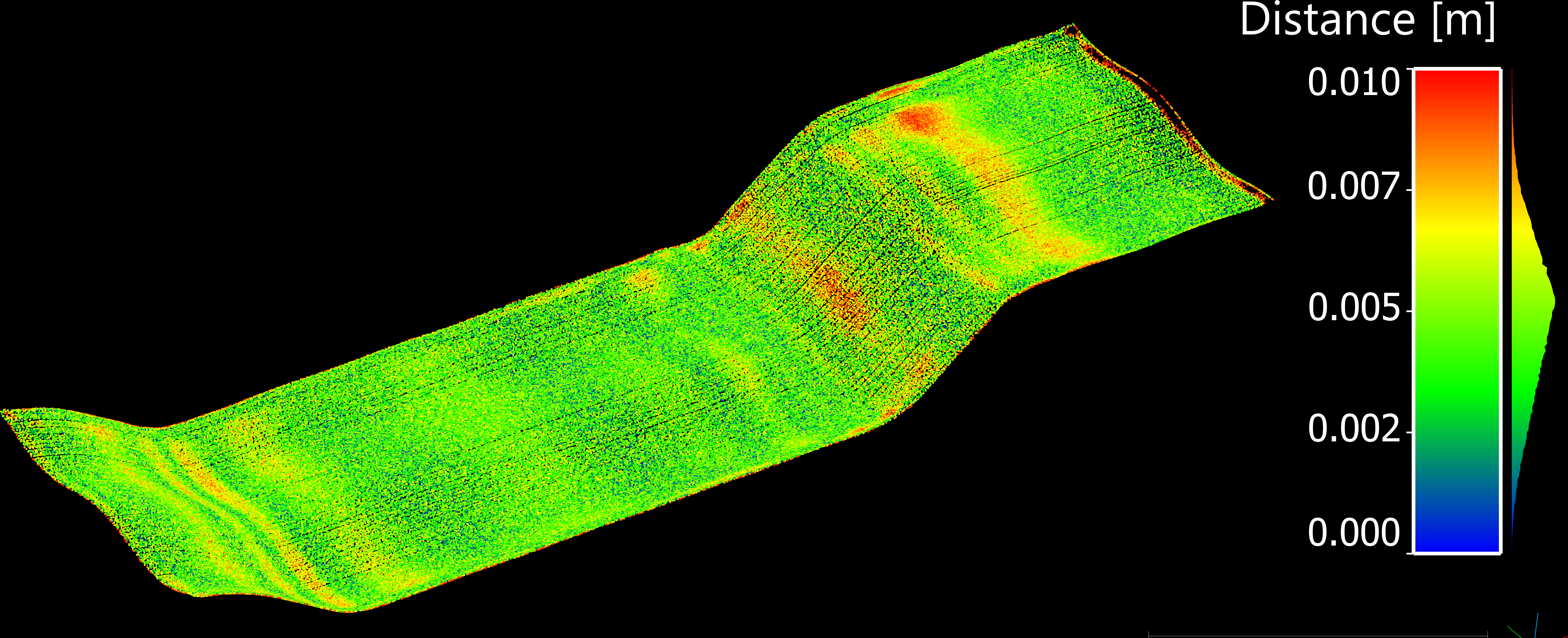
To assess model quality, we can look into model error as the spatial distance between the modeled point cloud and the ground truth, either represented as a 3D distance or separately along the X, Y, and Z axes. Of particular interest are the distribution, mean, and Root Mean Squared Error (RMSE) of this error. Fig. 18 illustrates the simulated PC generated by the survey simulator under conditions with zero measurement uncertainty. The points are color-coded according to the magnitude of the 3D model error, representing the distance between the estimated model and the ground truth. The mean model error in this scenario is 0.1 mm, with an RMSE of 3 mm, confirming that, despite being small, a model error clearly exists.
In the experiment, each point in the simulated dataset ends up with 1,000 realizations along the X, Y, and Z components. For each component, we compute the uncertainty value σ, defined as the standard deviation corresponding to the 68 % CL of the distribution. As described in Section 4, the uncertainties are simulated based on the developed uncertainty model in Section 2. Convergence of the Monte Carlo simulations was assessed by monitoring the stability of the estimated mean and standard deviation over increasing numbers of iterations. Statistical metrics stabilized after approximately 800–1,000 iterations, confirming that 1,000 simulations were sufficient. The selected surface modeling approach (MBA) represents a 2.5D model. Like other 2.5D DBMs, its primary emphasis lies on uncertainty in the vertical Z direction. To better visualize and evaluate the impact of vertical uncertainties, we chose uncertainty values of approximately (0.02, 0.02, 0.06) m for position (XPose, YPose, ZPose) components, respectively. Notice that ratio of the positional uncertainty to vertical one is lower than the real data in the simulation. This was done to minimize the influence of large horizontal positioning errors and better isolate and assess the effect of the modeling process on the vertical (z) component, which was the main focus of this study. The horizontal uncertainties were kept at low levels to avoid masking or distorting the analysis of vertical uncertainty propagation. Fig. 19 illustrates these uncertainties separately for each component (X, Y, and Z) and for each point individually. Fig. 19 provides an XY view of the simulated data points, color-coded according to uncertainty magnitude. It clearly shows that the uncertainty in the Z component (height) is dominant compared to X and Y. In Fig. 19d we see the combined standard uncertainty of the MC simulations. In which the uncertainty is calculated as,
 |
(18) |
It is important to note that the difference between this uncertainty measure and the TPU values is that TPU refers specifically to extended uncertainties, which are calculated by Eqs. 9 and 10.
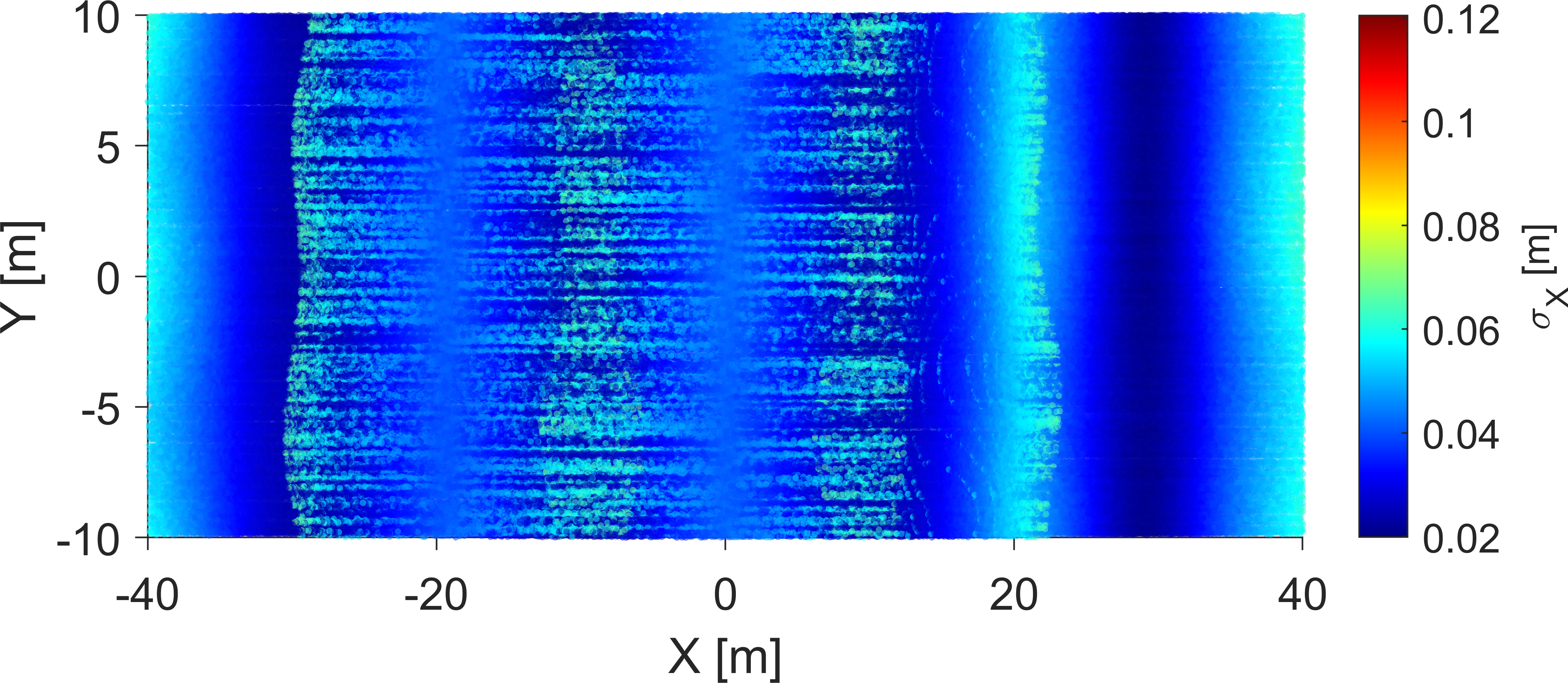

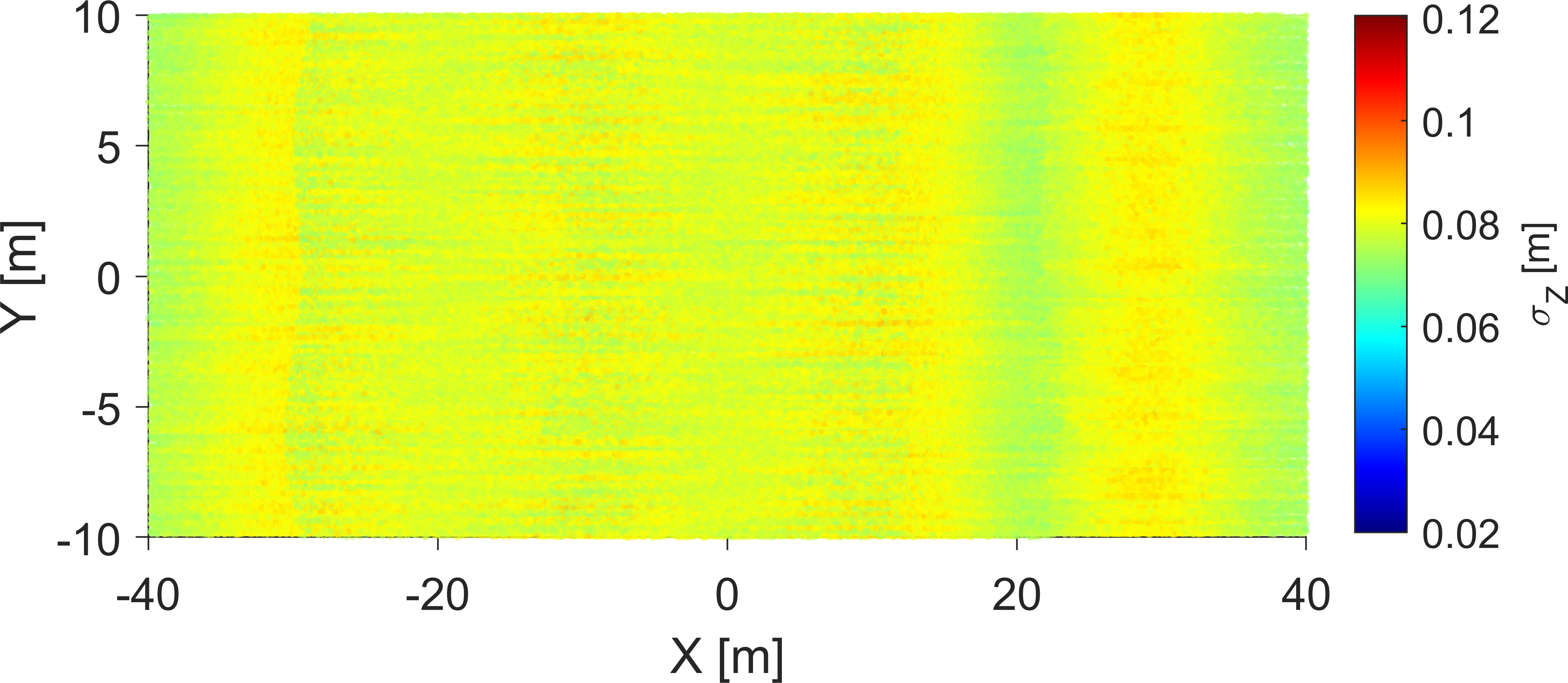
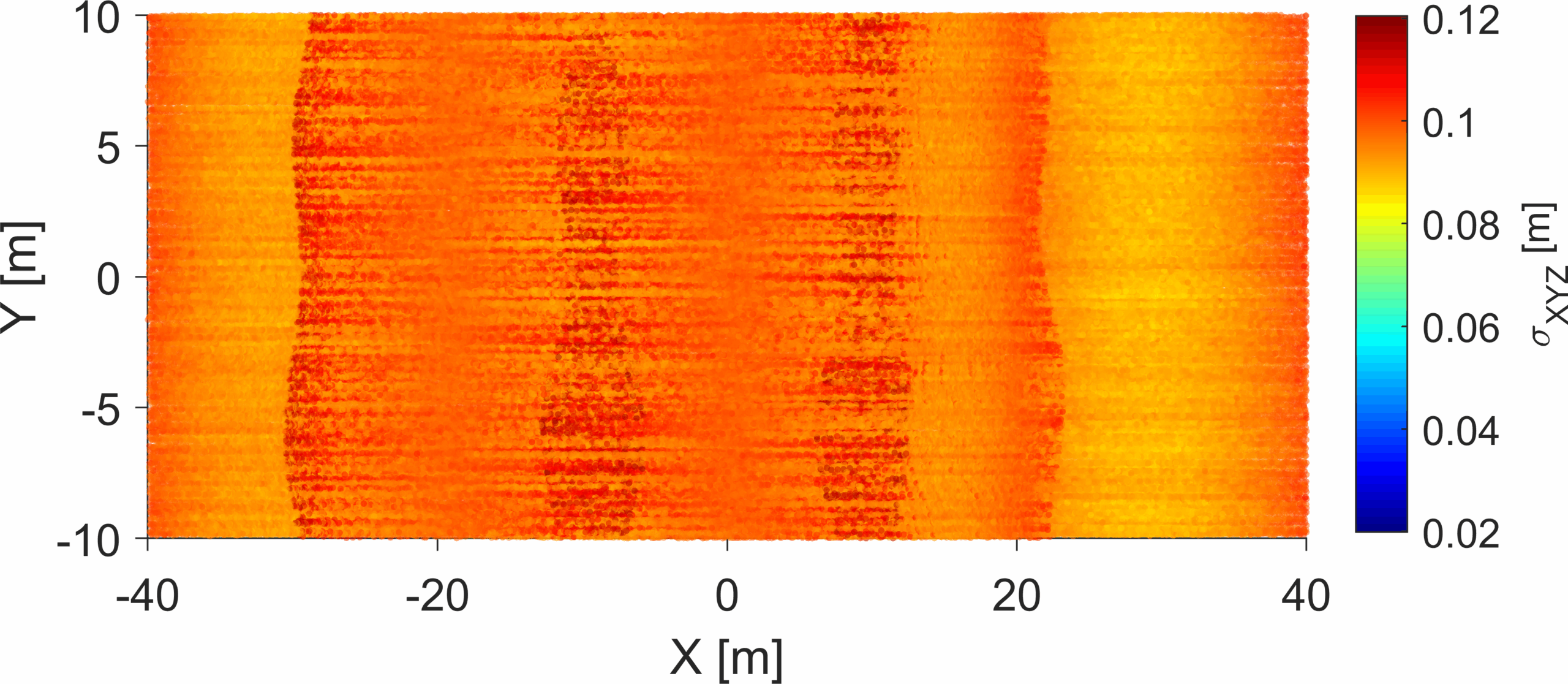
This uncertainty information is utilized to construct the weight matrix required for the GMM adjustment. It’s important to note that the MBA model is essentially a 2.5D representation, with parameters estimated by minimizing errors specifically in the Z-direction. MBA inherently cannot fully capture or exploit the complete 3D structure of positional uncertainties. This modeling simplification may lead to some loss of fidelity, particularly when significant horizontal errors are present. Consequently, for constructing the weight matrix, we primarily use the estimated uncertainty σZ, as shown in Fig. 19c (refer to Eq. 15). However, in reality – as well as in our simulations – uncertainty exists in all three spatial dimensions. Even though the MBA model does not explicitly estimate parameters in the X and Y directions, uncertainties in these dimensions can still impact model quality. For this reason, we also explore a scenario in which observations are weighted based on the combined uncertainty σXYZ. In total, we consider three scenarios in our analysis:
- Case 1: No weighting applied during adjustment
- Case 2: Observations weighted based only on vertical uncertainty σZ (Eq. 15)
- Case 3: Observations weighted using full 3D uncertainty σXYZ (Eq. 18)
Comparing these three scenarios allows us to assess not only the general effectiveness of applying uncertainty-based weights but also whether including full 3D uncertainties can meaningfully improve our results for a model inherently focused on vertical accuracy.
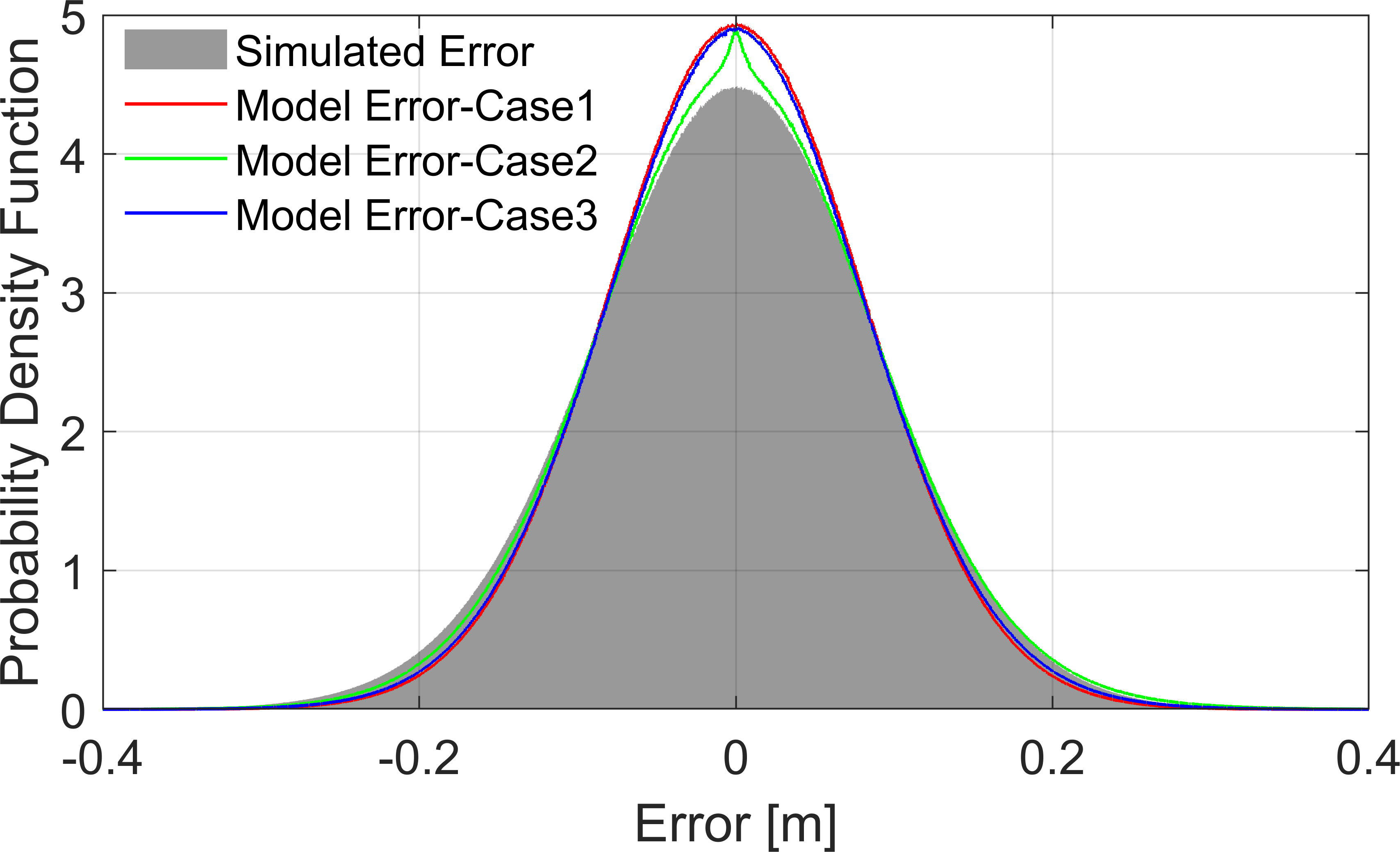
Here, we further investigate the Monte-Carlo simulation results, specifically examining the detailed distribution of errors. We consider both the adjustment quality and the difference between the estimated model and ground truth. The adjustment quality is evaluated using the residual differences between observations and the estimated model, quantified by root of a posteriori variance factor 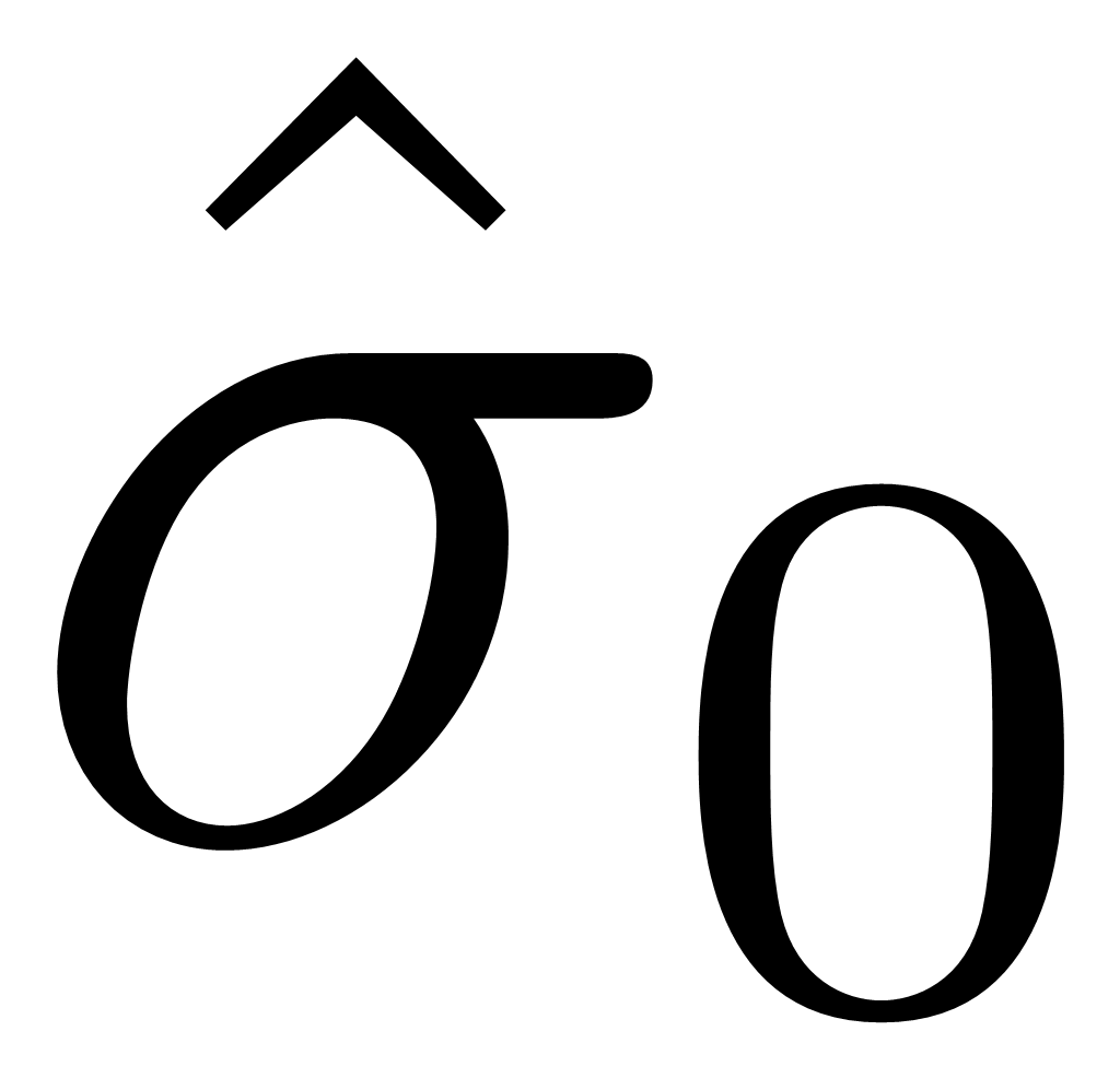 (see Eq. 17). These error distributions are presented in Fig. 20.
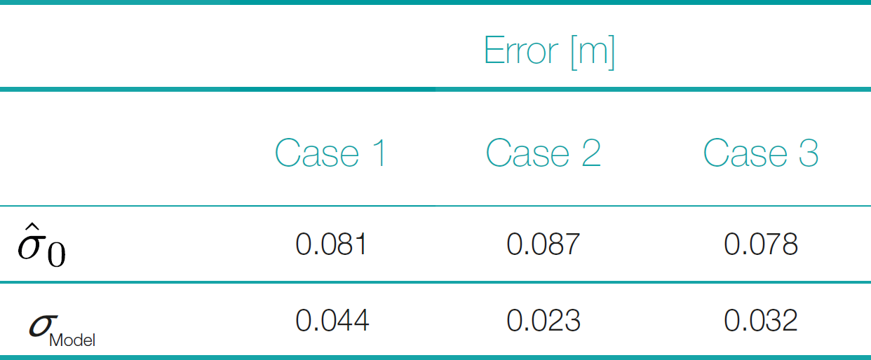
The gray histogram represents the distribution of simulated errors, specifically the vertical (Z-direction), distances between simulated points and the ground truth. This distribution is approximately normal, with an RMSE of 0.09 m. The error distributions from all three modeling scenarios align closely with the simulated error distribution, indicating that each scenario effectively captures the error structure. Furthermore, all three adjustment scenarios yield very similar values for the a-posteriori variance factor: 0.081 m, 0.087 m, and 0.078 m for Cases 1, 2, and 3, respectively. These nearly identical values suggest that the application of weights, whether based solely on vertical uncertainty or combined 3D uncertainty, does not significantly impact the overall adjustment quality.
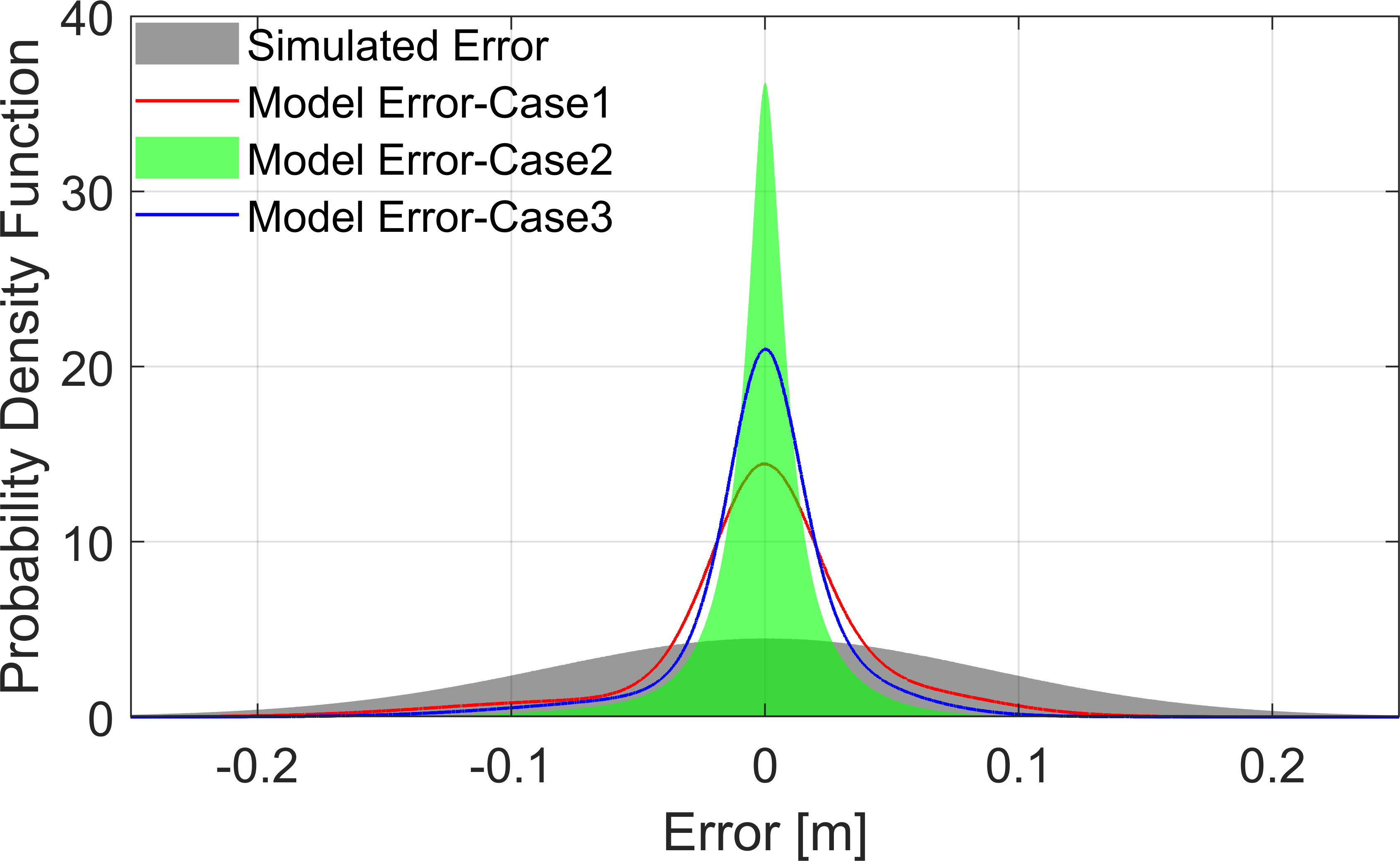
We further assess model quality by evaluating the difference between the estimated model and the ground truth, specifically the vertical (Z-direction), quantified by RMSE of these errors σModel. Fig. 21 presents the corresponding distributions of these errors for all three cases. In each scenario, the model error is consistently less than half of the a-posteriori variance factor , indicating that the estimated model gives a much better estimation of the ground truth. The unweighted scenario (Case 1) has the largest error, with σModel = 0.044 m, and its distribution shows clear asymmetry, suggesting the presence of bias. Introducing weighting significantly reduces the error and improves symmetry in the distribution. Case 2, weighted by vertical uncertainty σZ, achieves the smallest model error, σModel = 0.023 m, demonstrating a narrower and more symmetric distribution. Case 3, weighted by full 3D uncertainty σXYZ, also shows substantial improvement over the unweighted case (σModel = 0.032 m), although its error reduction is slightly less pronounced than in Case 2. These quantitative results are summarized in Table 2. These results highlight that applying uncertainty-based weighting enhances model quality by reducing bias and improving error symmetry. Interestingly, the slightly better performance of Case 2 compared to Case 3 might stem from the inherent nature of the MBA approach as a 2.5D modeling method, which primarily optimizes vertical accuracy. Although considering full 3D uncertainties (Case 3) clearly benefits the model, the inherent vertical emphasis of the MBA model means that its greatest accuracy gains come specifically from weighting by vertical uncertainties. This improves overall results in terms of distribution characteristics, and error symmetry. These subtle improvements in modeling accuracy, summarized in Fig. 21, underscore the importance of selecting appropriate uncertainty weighting – even when ground-truth data are unavailable and biases might otherwise remain unnoticed.
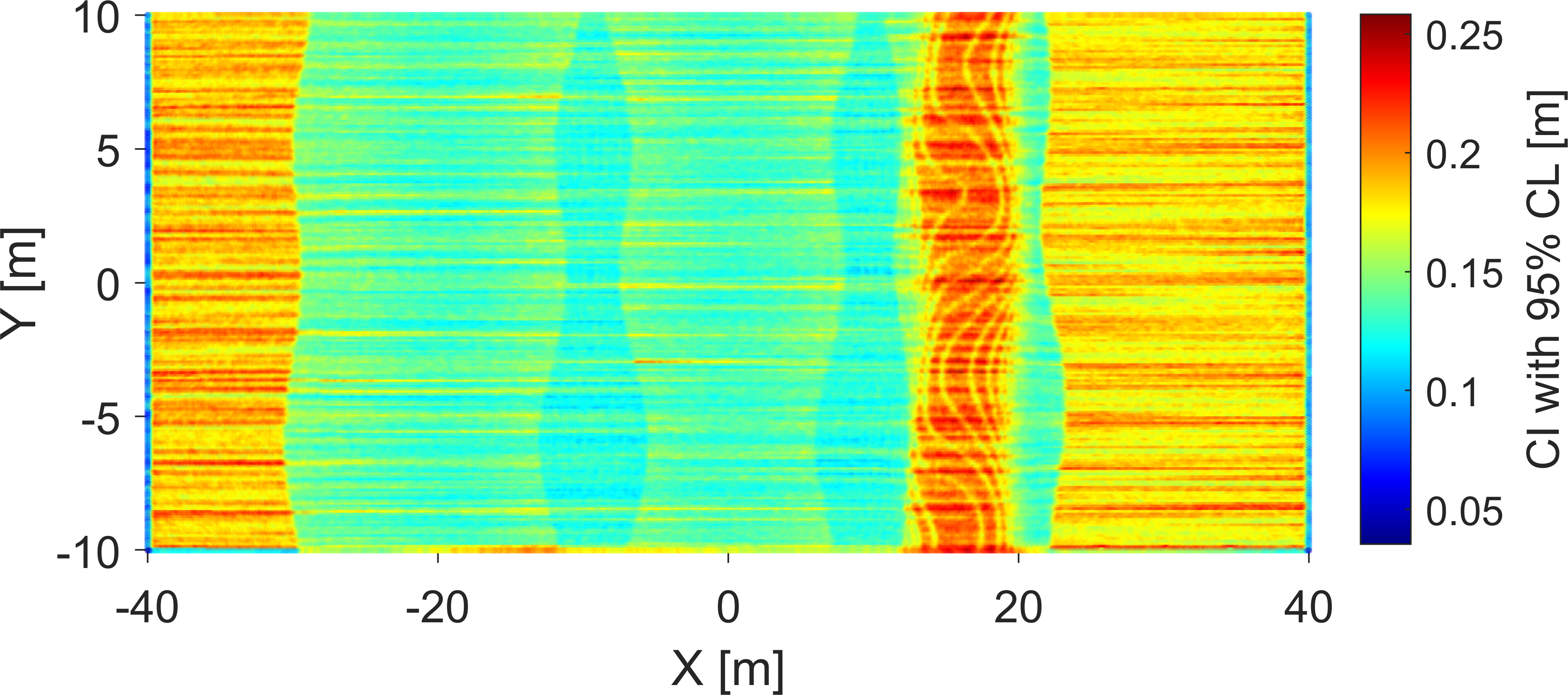
We further leverage the Monte-Carlo simulation results to create CI, enabling us to produce a detailed assessment of model quality. Each simulated realization generates slight variations in modeled values at each point, and by analyzing these variations, we can derive a meaningful CI. Fig. 20 illustrates a CI with a 95 % CL. The figure shows an XY view of the modeled area, with each point color-coded according to the length of its CI.
Comparing this CI map to the uncertainty distribution in Fig. 22, we observe an interesting difference: while the original uncertainties are highest near the edges of each survey swath – primarily due to unfavorable measurement angles – the modeled CIs are actually lower in these boundary regions. This apparent discrepancy arises because the boundaries of adjacent swaths overlap, providing redundant observations that help reduce the uncertainty and improve modeling accuracy, despite initially poorer measurement quality due to higher incidence angles. Thus, these overlapping areas offer enhanced information density, resulting in a higher-quality model with smaller uncertainties, even where individual measurements originally exhibited higher uncertainty.
These CI maps highlight areas with sufficient data coverage and indicate critical regions where data reliability might otherwise be overlooked. This provides users with a powerful visual tool for decision-making, aiding in strategic interpretation and effective risk identification. The generated CI maps have several practical applications. For survey planning, realistic simulation of measurement uncertainty allows surveyors to predict coverage quality, identify areas where higher uncertainties are expected, and optimize survey parameters such as vessel routes, ping rates, and swath overlap. In terms of confidence mapping, the method produces detailed spatial uncertainty maps that incorporate both measurement and modeling errors, allowing users to generate IHO S-44 compliance layers or internal quality indicators for the delivered bathymetric products. Furthermore, for real-time QA/QC, the approach could be adapted to provide near real-time estimates of expected uncertainty during data acquisition. This would allow operators to dynamically adjust survey settings if quality thresholds are not being met.
6 Conclusion
This study is divided into two parts. In the first part, we developed and evaluated a model to predict uncertainties for a hydrographic survey system. Although the measurement model was designed for a specific survey vessel, the underlying concept and workflow are adaptable to other systems equipped with MBES. Our analysis involved defining uncertainty measures according to classical GUM guidelines and conducting extensive Monte-Carlo simulations. The results indicated strong agreement between the two methods, confirming their consistency. However, MCM offers notable advantages over the classical approach, which is less effective for highly nonlinear measurement models and requires complex partial derivatives, MCM accommodates various PDF distributions and provides uncertainty estimates directly as a complete PDF, enabling more extensive analysis. To validate our developed uncertainty model, we compared its results to those obtained from a commercial software solution. Although the overall uncertainty patterns were generally compatible, systematic deviations were observed, likely due to differences in model parameters and assumptions. These discrepancies, however, do not compromise the primary goal of generating relative weights for subsequent modeling steps, ensuring that the later analyses remain robust and reliable.
In the second part of the study, we developed a survey simulator to generate measurements that incorporate uncertainties derived from our model. This controlled environment allowed us to validate the modeled data against known ground-truth values. Using a Monte-Carlo experiment, we assessed the quality of DBMs by incorporating uncertainty information to weight observations during modeling. The results demonstrated that integrating accurate uncertainty information improved the overall accuracy and reliability of the models. Although the numerical improvements may be subtle, they significantly enhance confidence in the resulting models. Additionally, the uncertainty data facilitated the creation of quality maps accompanying the DBMs, which effectively highlight regions of varying reliability and provide practical guidance for future survey planning and data interpretation. The generalizability of the simulation framework depends on the validity of the underlying physical models for uncertainty estimation (e.g., Hare, 1995; Wirth, 2011). Significant variations in measurement conditions or system behavior may require adjustment of simulation parameters or model structures to maintain accuracy.
While in this study we used synthetic surfaces to provide a precisely controlled ground truth, future work should explore the application of the proposed uncertainty modeling framework to real-world surfaces derived from dense MBES surveys. This would allow evaluation of model performance under more realistic and complex seabed conditions.
Further investigation of this experiment using a full 3D surface model is recommended. While the MBA model effectively represents 2.5D surfaces, it does not fully capture or propagate full 3D positional uncertainties. This limitation may constrain the fidelity of uncertainty integration, particularly in environments with strong three-dimensional variability. Further investigation using a full 3D surface model and comprehensive 3D uncertainty propagation is recommended. The application of a comprehensive 3D model, along with full-scale 3D uncertainties, has the potential to yield more profound insights into the manner in which uncertainty information influences model performance and accuracy. This analysis could more effectively reveal the benefits of incorporating uncertainties directly into the modeling process.
References
Abubakar, A. A. and Poerbandono, P. (2023). Effectiveness of vertical error budget model for portable multi-beam echo-sounder in shallow water bathymetric survey. IOP Conference Series: Earth and Environmental Science, 1245(1):012041. https://doi.org/10.1088/1755-1315/1245/1/012041
Alkhatib, H., Neumann, I. and Kutterer, H. (2009). Uncertainty modeling of random and systematic errors by means of Monte Carlo and fuzzy techniques. Journal of Applied Geodesy, 3, pp. 67–79. https://doi.org/10.1515/JAG.2009.008.
Arnold, J. and Shaw, S. (1993). A surface weaving approach to multibeam depth estimation. Proceedings of OCEANS’93. II–95.
Benning, W. (2011). Statistik in Geodäsie, Geoinformation und Bauwesen (4. Aufl.). Berlin, Offenbach: Wichmann.
BFG (2013). Neue Entwicklungen in der Gewässervermessung. Kolloquium am 20./21. November 2012 in Koblenz. – Veranstaltungen 5/2013, Koblenz, Mai 2013, 104 S. https://doi.org/10.5675/BfG_Veranst_2013.5
Bisquay, H., Freulon, X., De Fouquet, C. and Lajaunie, C. (1998). Multibeam data cleaning for hydrography using geostatistics. IEEE Oceanic Engineering Society. OCEANS’98. Conference Proceedings (Cat. No.98CH36259). pp. 1135–1143. https://doi.org/10.1109/OCEANS.1998.724413
Bjørke, J. T. and Nilsen, S. (2009). Fast trend extraction and identification of spikes in bathymetric data. Computers & Geosciences 35, pp. 1061–1071. https://doi.org/10.1016/j.cageo.2008.05.009
Bottelier, P., Briese, C., Hennis, N., Lindenbergh, R. and Pfeifer, N. (2005). Distinguishing features from outliers in automatic Kriging-based filtering of MBES data: a comparative study. In P. Renard and H. Demougeot-Renard (Eds.), Geostatistics for environmental applications (pp. 403–414). Berlin and Heidelberg: Springer. https://doi.org/10.1007/3-540-26535-x_ 34
Bureick, J., Alkhatib, H. and Neumann, I. (2016). Robust Spatial Approximation of Laser Scanner Point Clouds by Means of Free-form Curve Approaches in Deformation Analysis. Journal of Applied Geodesy, 10, pp. 27–35. https://doi.org/10.1515/jag-2015-0020
Delaunay, B. (1934). Sur la sph6re vide: Bull, Acad. Science USSR VII, Clas. Sci. Mat. Nat, pp. 793–800.
Eakins, B. W. and Taylor, L. A. (2010). Seamlessly integrating bathymetric and topographic data to support tsunami modeling and forecasting efforts. Ocean globe, pp. 37–56.
Erdogan, S. (2009). A comparision of interpolation methods for producing digital elevation models at the field scale. Earth Surface Processes and Landforms, 34: pp. 366–376. https://doi.org/https://doi.org/10.1002/esp.1731
Haji Mohammadloo, T., Snellen, M. and Simons, D. G. (2018). Multi-beam echo-sounder bathymetric measurements: Implications of using frequency modulated pulses. The Journal of the Acoustical Society of America, 144, pp. 842–860. https://doi.org/10.1121/1.5050816
Haji Mohammadloo, T., Snellen, M., Amiri-Simkooei, A. and Simons, D. G. (2019). Assessment of reliability of multi-beam echo-sounder bathymetric uncertainty prediction models. Proceedings of the 5th Underwater Acoustics Conference and Exhibition, pp.783–790, Crete, Greece.
Hare, R. (1995). Depth and Position Error Budgets for Mulitbeam Echosounding. The International Hydrographic Review, 72(2), https://journals.lib.unb.ca/index.php/ihr/article/view/23178 (last accessed 4 May 2025).
Hare, Rob, Eakins, B. W. and Amante, C. J. (2011). Modelling Bathymetric Uncertainty. The International Hydrographic Review, 6. https://journals.lib.unb.ca/index.php/ihr/article/view/20888 (last accessed 4 May 2025).
Harris, C. R., Millman, K. J., van der Walt, S. J., Gommers, R., Virtanen, P., Cournapeau, D., Wieser, E. et al. (2020). Array programming with NumPy. Nature (Springer Science and Business Media LLC), 585, pp. 357–362. https://doi.org/10.1038/s41586-020-2649-2
IHO (2022). Standards for Hydrographic Surveys (ed. 6.1). IHO Special Publication S-44, International Hydrographic Organization, Monaco. https://iho.int/uploads/user/pubs/standards/s-44/S-44_Edition_6.1.0.pdf (last accessed 4 May 2025).
ISO/GUM (1995). Guide to the Expression of Uncertainty in Measurement. Standard, International Organization for Standardization, Geneva, CH.
ISO/GUM (1998). Guide to the Expression of Uncertainty in Measurement (GUM) – Supplement 1: Numerical Methods for the Propagation of Distributions. Standard, International Organization for Standardization, Geneva, CH.
Lee, S., Wolberg, G. and Shin, S. Y. (1997). Scattered data interpolation with multilevel B-splines. IEEE transactions on visualization and computer graphics, 3, pp. 228–244.
Lorenz, F., Artz, T., Brüggemann, T., Reich, J., Weiß, R. and Winterscheid, A. (2021). Simulation-based evaluation of hydrographic data analysis for dune tracking on the River Rhine. PFG–Journal of Photogrammetry, Remote Sensing and Geoinformation Science, 89(2), pp.111–120.
Maleika, W. (2013). The influence of track configuration and multibeam echosounder parameters on the accuracy of seabed DTMs obtained in shallow water. Earth Science Informatics, 6, pp. 47–69. https://doi.org/10.1007/s12145-013-0111-9
Maleika, W., Palczynski, M. and Frejlichowski, D. (2012). Effect of Density of Measurement Points Collected from a Multibeam Echosounder on the Accuracy of a Digital Terrain Model. In J.-S. Pan, S.-M. Chen and N. T. Nguyen (Eds.), Intelligent information and database systems (pp. 456–465). Berlin: Springer. https://doi.org/10.1007/978-3-642-28493-9_ 48
Maune, D. F., Kopp, S. M., Crawford, C. A. and Zervas, C. E. (2007). Digital elevation model technologies and applications: The DEM users manual. Bethesda, MD: American Society for Photogrammetry and Remonte Sensing, ASPRS.
Mohammadivojdan, B, Alkhatib, H., Brockmeyer, M., Jahn, C.-H. and Neumann, I. (2020). Surface Based Modelling of Ground Motion Areas in Lower Saxony. Institutionelles Repositorium der Leibniz Universität Hannover. https://doi.org/10.15488/9344
Mohammadivojdan, B., Brockmeyer, M., Jahn, C.-H., Neumann, I. and Alkhatib, H. (2021). Regional Ground Movement Detection by Analysis and Modeling PSI Observations. Remote Sensing, 13, 2246. https://doi.org/10.3390/rs13122246
Mohammadivojdan, B., Lorenz, F., Artz, T., Weiß, R., Hake, F., Alkhatib, Y., Neumann, I. and Alkhatib, H. (2024). Robust algorithm for automatic surface-based outlier detection in MBES point clouds. Marine Geodesy, 48(2), pp. 141–172. https://doi.org/10.1080/01490419.2024.2408684
Paquet, R. (2010). Estimation of interpolation error in DEMs using statistical methods. FIG Congress 2010 – Facing the Challenges–Building the Capacity.
Piegl, L. (1997). The NURBS Book (2nd ed.). Berlin and Heidelberg: Springer. https://doi.org/10.1007/978-3-642-59223-2
QPS (2025). QPS QINSy. https://qps.nl/qinsy/ (last accessed 10 March 2025).
Rishikeshan, C. A., Katiyar, S. K. and Vishnu Mahesh, V. N. (2014). Detailed Evaluation of DEM Interpolation Methods in GIS Using DGPS Data. 2014 International Conference on Computational Intelligence and Communication Networks, pp. 666–671. https://doi.org/10.1109/CICN.2014.148
Schwarz, W. (2020a). Methoden zur Bestimmung der Messunsicherheit nach GUM – Teil 1. AVN Allgemeine Vermessungs-Nachrichten, pp. 69–86.
Schwarz, W. (2020b). Methoden zur Bestimmung der Messunsicherheit nach GUM – Teil 2. AVN Allgemeine Vermessungs-Nachrichten, pp. 211–219.
Sullivan, C. B. and Kaszynski, A. (2019). PyVista: 3D plotting and mesh analysis through a streamlined interface for the Visualization Toolkit (VTK). Journal of Open Source Software, 4, 1450. https://doi.org/10.21105/joss.01450
Tengku A., Afrizal, T., Abbas, M. A., Mustafar, M. A., Said, M. S. M., Hashim, N. M. and Sulaiman, S. A. (2022). Investigating the Vertical Uncertainty in MBES Measurements. 2022 IEEE 18th International Colloquium on Signal Processing & Applications (CSPA), pp. 431–435. https://doi.org/10.1109/CSPA55076.2022.9781857
Wirth, H. (2011). Messunsicherheiten in der Gewässervermessung [Tech. rep.]. BfG-Bericht 1734.
Wlodarczyk-Sielicka, M., Lubczonek, J. and Stateczny, A. (2016). Comparison of selected clustering algorithms of raw data obtained by interferometric methods using artificial neural networks. 2016 17th International Radar Symposium (IRS), pp. 1–5. https://doi.org/10.1109/IRS.2016.7497290
WSA (2023). Peilschiff Uwe Jens Lornsen. Wasserstraßen- und Schifffahrtsamt Elbe-Weser. https://www.wsa-elbe-nordsee.wsv.de/Webs/WSA/Elbe-Nordsee/DE/1_Wasserstrassen/4_SchiffeMaschinenwesen/UJLornsen/ujlornsen_node.html (last accessed 5 January 2024).
Yang, C.-S., Kao,S.-P., Lee, F.-B. and Hung, P.-S. (2004). Twelve different interpolation methods: A case study of Surfer 8.0. Proceedings of the XXth ISPRS congress, pp. 778–785.
Authors’ biographies

Bahareh Mohammadivojdan received her M. Sc. in Geodesy and Geoinformatics from Leibniz University Hannover in 2019 and is currently a researcher at the Geodetic Institute of the same university. Her work focuses on engineering geodesy and geodetic data analysis, with research interests including mathematical surface approximation, uncertainty modeling, and the analysis of geospatial data for hydrographic and topographic applications. https://orcid.org/0000-0002-0648-1162

Dr.-Ing. Frederic Hake pursued his studies in the field of geodesy and geoinformatics at Leibniz University Hannover. He was employed at the Geodetic Institute, Leibniz University Hannover, where he completed his doctorate in 2024, undertaking research in the field of damage detection in buildings using machine learning techniques. Since 2024 he has been employed by Allsat GmbH, where he has been engaged in a number of activities, including the monitoring of ground movements and the infrastructural monitoring of risk structures. https://orcid.org/0000-0001-7424-2270

Felix Lorenz graduated with an M. Sc. degree in Geodesy and Geoinformation from the University of Bonn in 2016. Currently he is working in the Department Geodesy and Remote Sensing of the Federal Institute of Hydrology in Germany as a member of the hydrographic survey working group. He gathered knowledge and experience in the field of dune tracking as a member of the research and development project MAhyD (morphodynamic analyses using hydroacoustic data). In his current position he works consulting the German Waterways and Shipping Administration concerning hydrographic data analysis and sensor specifications.

Jan Ole Böllert studied Geodesy and Geoinformatics at Leibniz University of Hannover. He graduated with a Master Thesis on “Uncertainty Modelling of Echosounder Measurements”. Since 2024 he is employed at the Saxon State Ministry of Infrastructure and Regional Development (SMIL) in Dresden for a technical traineeship for civil service in surveying.

Dr.-Ing. Robert Weiß graduated as geodesist from TU Dresden (Germany) in 2003. He investigated the comparability of water surface levels derived from tide gauges, GNSS stations at tide gauges and satellite altimetry and completed his PhD with the topic ‘Detection and description of sea level and its changes in the area of the German Bight’ in 2012. He has been working in the Federal Institute of Hydrology in Koblenz since 2005. His current work focuses on the evaluation of new sensors, measurement and evaluation methods in the context of digital terrain modeling, such as the analysis of red and green ALS flights.

Dr.-Ing. Thomas Artz graduated as geodesist from the University of Bonn. He conducted research in the field of Very Long Baseline Interferometry, Earth Rotation and Terrestrial Reference Frames and completed his PhD on Subdaily Earth Rotation Variations in 2011. Since 2022 he is head of the department of Geodesy and Remote Sensing at the Federal Institute of Hydrology in Koblenz. His department conducts R&D for geodetic and remote sensing tasks regarding the federal waterways in Germany and consults the German Waterways and Shipping Administration as well as the Federal Ministry for Digital and Transport in these research fields.
Univ.-Prof. Dr.-Ing. Ingo Neumann received his Dipl.-Ing. and Ph.D. in Geodesy and Geoinformatics at the Leibniz Universität Hannover in 2005 and 2009, respectively. Since 2012, he has been a Full Professor in the field of Engineering Geodesy and Geodetic Data Analysis at the Geodetic Institute of Leibniz Universität Hannover. His research areas are: artifical intelligence, adjustment theory and uncertainty models, multi-sensor systems, quality assessment, geodetic monitoring, terrestrial laser scanning, and automation of measurement processes. He is active in national and international scientific associations and an official delegate of the German and International Organization of Standardization (DIN and ISO). https://orcid.org/0000-0001-9110-7345

PD Dr.-Ing. Hamza Alkhatib studied Surveying Engineering at Karlsruhe Institute of Technology (KIT). He earned his PhD in 2007 from the University of Bonn with a dissertation on “Monte Carlo methods and their applications to satellite gravity missions”. Since 2007, he has been leading the research group for Expert-based Data Analysis and Quality Processes at the Geodetic Institute of Leibniz University Hannover. In 2020, he completed his Habilitation on “Advanced Methods and Algorithms for Computer-based Geodetic Data Analysis. His research focuses on machine learning, Bayesian modeling, Monte Carlo methods, and uncertainty quantification in geodetic data analysis. https://orcid.org/0000-0002-4480-1067