


Abstract
1 Introduction
The development of the terrestrial laser scanner is considered as a milestone in the enhancement of geodetic measuring instruments (Witte & Sparla, 2015). Through the transition from discrete to continuous area-wise measurements, the terrestrial laser scanner allows to capture entire objects instead of a few object points (Witte & Sparla, 2015). Installed on airborne and land-based platforms, terrestrial laser scanners can collect 3D data in large volumes with an accuracy of better than 1 cm while maintaining an unprecedented resolution and speed (Shan & Toth, 2018). Subsequently, terrestrial laser scanners have become well established surveying techniques for the acquisition of geospatial information. Hence, the retrieved point clouds are not only used to produce digital terrain and 3D city models, but also in the scope of forest management and monitoring, the revamping of industrial installations as well as the documentation of cultural heritage sites (Vosselman & Maas, 2010). Next to the strong interest in capturing 3D objects on the landside, this interest has also been projected onto the water-, particularly the underwater side (Hildebrandt et al., 2008). Here, underwater infrastructure elements, such as port facilities, offshore wind turbines, pipelines, submarine cables and drilling platforms, require regular inspection, maintenance and repair (IMR) operations (Nauert & Kampmann, 2023). Driven by the potential to operate terrestrial laser scanners on water-based platforms such as unmanned vehicles or vessels to capture the surrounding environment above water as well as the development of bathymetric laser scanners mounted on for instance drones, the development of laser scanners operating only under water has become a crucial challenge in recent years. Next to the development of systems which are based on the triangulation principle, lately two companies also developed systems based on the Time-of-Flight (ToF) principle (3D at Depth, 2025; Fraunhofer IPM, 2025). Because of the recent development of the ToF Underwater LiDAR System (ULi) by the Fraunhofer Institute for Physical Measurement Techniques (IPM), there are so far no studies which further investigate the suitability of ULi under laboratory as well as under non-laboratory conditions and which assess to which extend this particular underwater laser scanner can be considered as the monitoring solution the worldwide expansion of underwater infrastructure elements requires. To change this subject, ULi is tested in varying environments, including two laboratory basins as well as the river Elbe. For the latter, the multisensory survey vessel of the HafenCity University Hamburg (HCU) is used.
2 State-of-the-art
Over the past decades, different technologies to realize measurements under water have been developed. Subsequently, underwater structures can be captured by using optical technologies such as digital cameras which are commonly used to support the visual inspection carried out by divers (Sun et al., 2021). Related studies to capture coral reefs (Muhammad, 2024) or to document archaeological underwater sites (Calantropio & Chiabrando, 2024), outline two possible applications. Furthermore, an exemplarily study from Ottaviano et al. (2024) shows, that digital cameras can also be mounted on remotely operated or autonomous underwater vehicles which allows the inspection of objects within depths of a few hundred metre. Although digital cameras are cheap and easy to operate, studies also describe that the quality of the retrieved images, including the appearance of colours, is heavily degraded by poor light conditions and turbidity (Wang et al., 2024). In addition, Alsakar et al. (2024) outline, that the restoration and the enhancement of underwater images include subjective as well as objective methods. While the appliance of subjective image quality metrices is time-consuming and cost-intensive, objective image quality assessment techniques apply mathematical and statistical models which – however – also rely on the human visual system. Subsequently, objective measurement parameters are sparse. Therefore, information about underwater structures is commonly gathered by using acoustic technologies such as traditional sonar systems. Related studies involve the underwater inspection of bridge structures (Zhang et al., 2024) and archaeological sites (Lee et al., 2021). The advantage of acoustic systems is, that they are not sensitive to turbidity and thus allow for long operational distances of several thousand metres. The drawbacks are, that those systems measure comparably slow and inaccurate. Hence, only a resolution in the range of centimetres, can be achieved (Lekkerkerk & Theijs, 2011, pp. 58 and 84).
In terms of monitoring tasks for large built underwater structures, especially in shallow-waters, neither cost- and labour-intensive camera operations resulting in heavily degraded images nor slowly operating acoustic systems providing low resolutions, are suitable. Hence, fast operating technologies which are able to detect deformations in the dimension of millimetres, indicating damage at an early stage, are required. Facing the worldwide expansion of underwater infrastructure elements, the demand for a fast, precise and high-resolved monitoring solution becomes even more present (Nauert & Kampmann, 2023). Driven by the high propagation velocity as well as the achievable accuracy and resolution, active optical techniques, such as underwater laser scanners, deliver enormous potentials.
To determine the 3D position of points, underwater laser scanners either use triangulation principles or the ToF method. Besides the varying functionalities, the main differences lie in the achievable scan range and the depth resolution. Hence, McLeod et al. (2013) outline, that triangulation-based laser scanners provide a higher depth accuracy when operating in a range of less than 1 m. Above 2.5 m, ToF laser scanners are generally more accurate. On account of this, the depth resolution of a ToF laser scanner depends on the resolution of the time or the phase measurement and not on the scan distance. Subsequently, systems using the ToF technique offer a greater potential for the usage in turbulent dynamic water bodies where the presence of currents and waves hinder the underwater laser scanner from approaching the object of interest up to a distance of 1 m.
Until now, two companies have developed ToF underwater laser scanning systems. While 3D at Depth developed the ToF operating systems SL3, SL4, SL4n and SL6 (3D at Depth, 2025), the Fraunhofer IPM developed the underwater laser scanner ULi (Fraunhofer IPM, 2025). With the technical specifications provided by the manufacturer, namely a sampling frequency of 100 kHz, a scanning distance in the range of several metres and a precision in the order of sub-millimetre in clear waters (Fraunhofer IPM, 2024), ULi has the potential to meet the demands which come along with the worldwide expansion of underwater infrastructure elements.
3 Sensor Technology
The underwater laser scanner ULi consists of two major components, being a scanning unit and a processing unit.
3.1 Scanning Unit
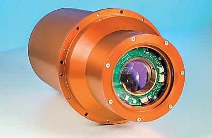
The waterproof cylindrical housing, illustrated in the Fig. 1, has a diameter of 0.172 m, a length of 0.375 m and can be used in depths of up to 300 m.
To emit short laser pulses in the order of one nanosecond onto the underwater environment and detect the returning light, a green laser with a wavelength of 532 nm and two rotating wedge prisms, allowing for a 44° field of view (FoV), are used. Hence, the distance to the target is determined based on the pulse propagation time. While the laser has a pulse repetition rate of 100 kHz, the rotating prisms allow the entire FoV to be captured without moving the underwater laser scanner. The laser pattern can be set to linear, circular or planar and thus dynamically adapted to the field of application (Fraunhofer IPM, 2024).
3.2 Processing unit
The hardware of ULi involves a processing unit. The backside of the processing unit contains inputs for a pressure sensor cable, a 24 V-DC power supply cable, an ethernet cable and a cable which is connected to the underwater scanning unit. The frontside features a pressure switch, a lock to start the scanner in the 3B mode, a laser-on-lamp indicating whenever the laser is used in the 3B laser mode and a power on / off switch. Hence, the laser scanner can be operated in two different laser modes, being laser class 2M and 3B. Since the laser radiation from the laser class 3B is dangerous for human eyes and skin, an additional pressure sensor is attached to the underwater laser scanner. Consequently, the laser operation in the 3B mode automatically switches off if the water level rises above a pre-defined pressure threshold of 0.7 dbar. This significantly enhances the safety at work. By connecting the processing unit with an ethernet cable to a PC or laptop, the entire operation and data acquisition of the underwater laser scanner can be steered over a graphical user interface (GUI). The GUI indicates the status of the scanning system and allows the user to set different parameters including the pulse rate or the laser pattern. Furthermore, the interface is used to start, record and stop the measurement. The measured data can be analysed by applying a full waveform analysis. Compared to a discrete signal analysis, this approach allows to separate the backscattered light-pulse from those caused by the water surface and particles within the water column. As a result of this separation, unwanted reflections within the signal can be suppressed and topographical data can be extracted (Hydro International, 2024).
4 Methodological approach
According to the information provided in Sections 2 and 3, ULi has the potential to become the monitoring solution the worldwide expansion of underwater infrastructure elements requires. To assess whether this potential can be realized, the following overall research question arises:
- Which performance and potential offers ULi?
To answer this question, the following sub-research question must be addressed:
- To which extent does the quality of the derived point clouds differ when ULi is tested under laboratory as well as under non-laboratory conditions?
In response to this sub-research question, three case studies were carried out:
- Static laboratory close-range measurements
- Static laboratory mid-range measurements
- Dynamic real-world close-range measurements
5 Case Studies
To evaluate the outcome of ULi, particular with regard to the achievable range and resolution, the conducted studies will be elaborated in the following sub-sections.
5.1 Static laboratory close-range measurements
To evaluate the close-range performance of ULi under laboratory clear water conditions, various static measurements in a test basin of the HCU, were carried out.
5.1.1 Test environment HCU Lab
The measurements were conducted in an already existing small acrylic glass basin with a length of 1.20 m, a width of 0.60 m and a depth of 0.60 m. The basin was filled with water from the tab to a water level of 0.45 m. To ensure a horizontal radiation of the measuring laser and thus a good impact angle on the target, a triangular substructure was established. With this set-up, which is also shown in the Fig. 2a, the distance between the lenses and the opposite end of the basin was approximately 0.56 m. To measure the turbidity of the water within the basin, the multi-sensor oceanographic profiler AML-3 from AML Oceanographic with a stated precision of 0.10 NTU, an accuracy of 0.20 NTU and a resolution of 0.01 NTU, was used (AML Oceanographic, 2025). The profiler indicated an average turbidity of 0.00 NTU, which means that the underwater laser scanner was tested under optimal conditions.
5.1.2 Targets HCU Lab
To assess the suitability of the underwater laser scanner with respect to different tasks, including IMR operations of different infrastructure elements, thirteen targets with varying surface characteristics were placed into the test basin. Hereby, also materials which are particularly used for the construction of underwater infrastructure elements, were selected. Subsequently not only a coated-, a lacquered- and a rusted steel plate, but for instance also two targets made out of wood, which was used in former times for the construction of quay walls and which is still used for the construction of mooring dolphins, were tested. While small targets were directly pressed onto the acrylic glass at the end of the basin, as shown in the Fig. 2b, targets which exceed the height of the basin were held approximately 5 cm in front of the glass rear panel.
As a result, it could not only be investigated whether the underwater laser scanner is suitable for inspection and maintenance operations on rusted quay walls and wooden mooring dolphins, but also to assess how varying surface textures, mainly characterized by their roughness, influence the reflection behaviour of the transmitted laser. Furthermore, the existing cracks, holes, scratches et cetera of the tested materials were used to assess whether ULi can technically be used to detect deformations in the range of millimetres. An overview of all targets and a more thoroughly elaboration can be derived from Walter et al. (2025).


5.1.3 Data acquisition HCU Lab
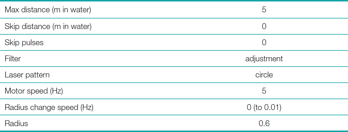
To conduct the measurements, the settings summarized in the following Table 1, were applied. To ensure that the target would be visible in the data, a maximum distance of 5 m and a skip distance of 0 m was set. Furthermore, the parameter skip pulses was set to 0. Considering that ULi measures 100.000 points per second and skipping none of the pulses, this resulted in a pulse repetition rate of 100 kHz. As the filter was set to adjustment, the green laser was emitted with a strength corresponding to the lowest possible laser class 2M. Hence, the reduction of the laser power increased the safety of work in the laboratory environment. To test the reflectivity behaviour of the different targets, a circular laser pattern, a motor speed of 5 Hz and a radius change speed of 0 Hz was applied. Hence, the laser rotated with a constant speed and at a constant radius on the surface of the target. To scan the entire surface of the targets, the radius change speed was adjusted to 0.01 Hz. In this case, the laser rotated with a firstly increasing and then decreasing radius and therewith captured the entire surface of the selected target. Since the smallest rotation radius occurs when setting the radius to 0.6, this parameter was selected.
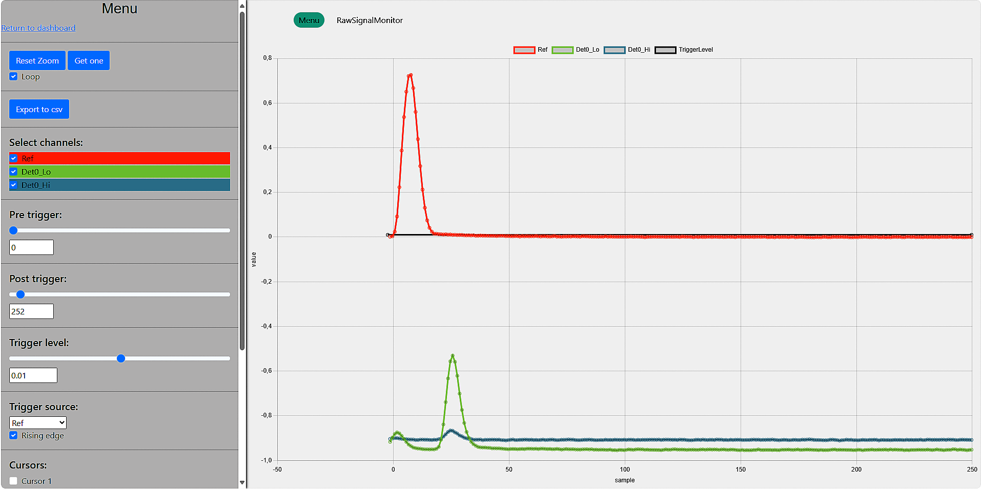
The incoming waveforms were directly reviewed in real-time using the Raw Signal Monitor. As it can be seen in the illustrated example in the Fig. 3, the live monitor displays three curves. The red curve refers to a fibre reference which is recorded before the light leaves the scanner. Thus, it functions as an internal reference signal. Once the light is transmitted and reflected, it reaches a detector where an avalanche photodiode converts the optical signal into an electrical signal. The electrical signal is split by a ratio of 1:10 between two amplifiers. Subsequently, the signal is strengthened to varying degrees. While the signal, which is attenuated by a factor of 10, is denoted as the sensitive channel and coloured in green, the other signal is denoted as rough or less sensitive channel and coloured in blue. Consequently, the green coloured signal is much more sensible.
In Fig. 3, the first peak of the green coloured curve indicates the reflection of the green laser on the lenses of the scanning unit while the second peak refers to the reflection triggered from the target. To assess the distance between the lenses of the underwater laser scanner and the target, the number of samples between the first and the second peak can be determined. Since each sample has a length of approximately 2.20 cm, the sample difference from the x-axis must be multiplied with this length. The derived product can be used to estimate the distance between the scanner and the target and to verify the curves displayed in the raw signal monitor. In the shown case, the estimated target distance is 0.44 m, which is regarded as realistic.
5.1.4 Results from HCU Lab
The retrieved waveforms were processed in Pulsalyzer and CloudCompare. Pulsalyzer is a proprietary post-processing software solution developed by the Fraunhofer IPM which can be used to review the derived waveforms, assess the associated point cloud and export the data from the proprietary .lidar format into .las files. The .las files can be imported into other point cloud processing software’s. For the purpose of this research, the open source point processing software CloudCompare was used.
Overall, the measurements show, that light coloured targets with a shiny smooth surface exhibit a better reflectivity and cause less scattering in comparison to dark coloured, matt and rough surfaces (Walter et al., 2025). The scattering of the point clouds, defined by their thickness, ranged from 6 mm to 48 mm which is significantly higher to what can be typically derived from terrestrial laser scanners. This might be related to the fact that the targets were held by hand and not securely fixed. Three exemplarily point clouds are shown in the Fig. 4 below. Since the water in the test basin was only 0.45 m deep, the increasing radius caused the green laser to be reflected on the calm water surface. This additional reflection is indicated by the horizontal line in all three point clouds. The additional visible concentric circular pattern is a result of the selected scan pattern “Circle”. As it can be seen in the left and in the middle point cloud, the holes within the selected target materials are clearly visible. To determine the diameter of the holes, a digital calliper with a stated resolution of 0.01 mm was used. While the holes in the white lacquered steel plate ranged from 5.20 mm to 6.09 mm, the holes of the black coated steel target ranged from 6.59 mm to 6.71 mm. For organic structures such as the wooden box, elements such as knotholes and grains are mainly recognized by their change in intensity. Nevertheless, the 30 cm long and 2.36 mm wide vertical notch in the centre of the target is visible. Subsequently, the static laboratory measurements show, that the close-range point clouds can be used to identify man-made structures such as drilled holes or cracks as well as organic structures down to the millimetre scale (Walter et al., 2025).

5.2 Static laboratory mid-range measurements
To evaluate the mid-range performance of ULi under clear water conditions, additional tests in the laboratory infrastructure of the Institute of Mechanics and Ocean Engineering (MUM) from the Technical University Hamburg (TUHH) were carried out.
5.2.1 Test environment MUM TUHH Lab
The tests were conducted in a 15 m long, 1.50 m wide and 1.60 m deep glass basin which was filled with water from the tab to a water level of 1.20 m. To allow for a maximum possible distance between the lenses and the opposite end of the basin, the underwater laser scanner was placed at one end of the basin. To ensure a horizontal radiation of the measuring laser and thus a good impact angle on the target, a construction made out of aluminium profiles and a tensioning strap was used. As a result, the centre of the lenses was roughly 0.64 m submerged under the water and the distance to the end of the basin was about 9 m. The oceanographic profiler indicated an average turbidity of 0.00 NTU, which means that the underwater laser scanner was again tested under most favourable conditions.
5.2.2 Targets MUM TUHH Lab
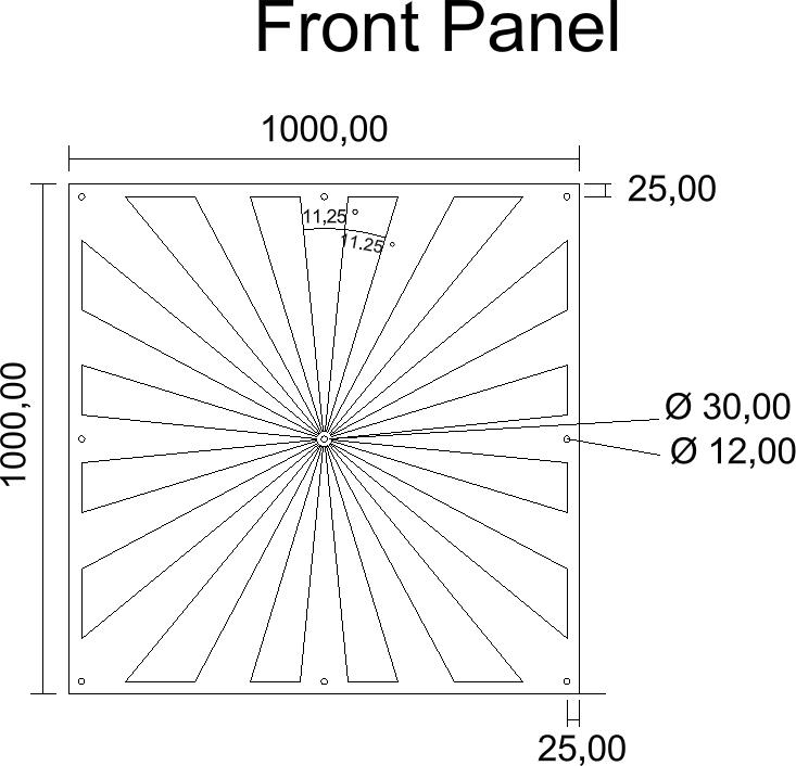
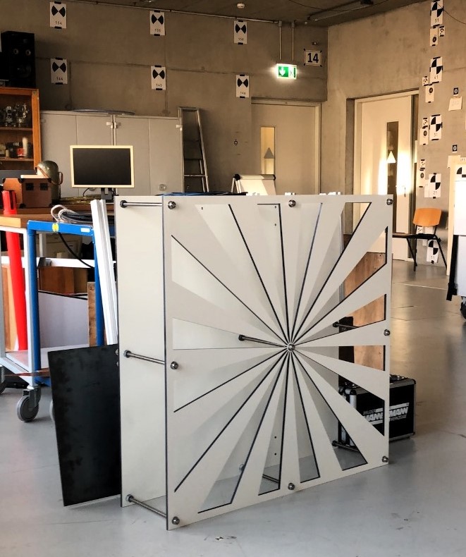
To further assess the performance of ULi and to make a conclusive statement about how wide a crack in a material must be to be clearly identified in the point cloud, the achievable resolution was further investigated. From the perspective of the user, the resolution describes the capability of the underwater laser scanner to detect small objects or object parts in a point cloud. Technically, this capability is influenced by the smallest possible angular increment between two successive points as well as the size of the laser spot on the object itself (Boehler et al., 2003). Hence, a test object which comprises small elements or narrow slots on a flat surface can help to determine application-specific resolution capabilities. As a result, a so-called Böhler star was constructed. To determine the best suitable construction material for underwater applications, the results from the first study described in Section 5.1, were examined. By means of that, not only the quality of the derived point cloud, mainly given by its scattering, but also the suitability of the material as such, including its weight and its thickness, were taken into consideration. Conclusively, the material Resopal was selected. To assess the size and the distribution of the rays for the front panel, the beam diameter of ULi and the beam divergence, which the Fraunhofer IPM specified with 2.00 mm at exit and 1.50 mrad respectively, were accounted. An information about the smallest angular increment of ULi was not available. Finally, a Böhler star consisting of 32 rays with a respective opening angle of 11.25° and a size of 1 m × 1 m was designed. The related drawing is shown in the following Fig. 5a. To mill the rays into the front Resopal panel, a S3 Cutter from Zünd with a stated resolution of
0.005 mm and a repetition accuracy of ± 0.03 mm, was used (Zünd, 2023). Since the target had to be stencilled once, it can be assumed that the overall Böhler star was manufactured with a final production quality of 0.20 mm.
If ULi offers a high resolution, driven by small angular increments and a narrow laser spot size, reflections should not only occur on the front, but also on the rear panel. If the reflections on the rear panel are present in the outer regions as well as close to the centre, a very high resolution is achieved (Boehler et al., 2003). Subsequently, the Böhler star can be used to gather resolution information from different ranges. To further investigate the influence that a changing panel to panel distance might have, the front and the rear panel of the Böhler star were connected by using nine 30 cm long threaded rods. The rods did not only allow to vary the distance between 1.16 cm and 24.90 cm, but also to enhance the overall stability of the Böhler star. The final assembly of all components was done by hand and is illustrated in the Fig. 5b.
5.2.3 Data acquisition MUM TUHH Lab
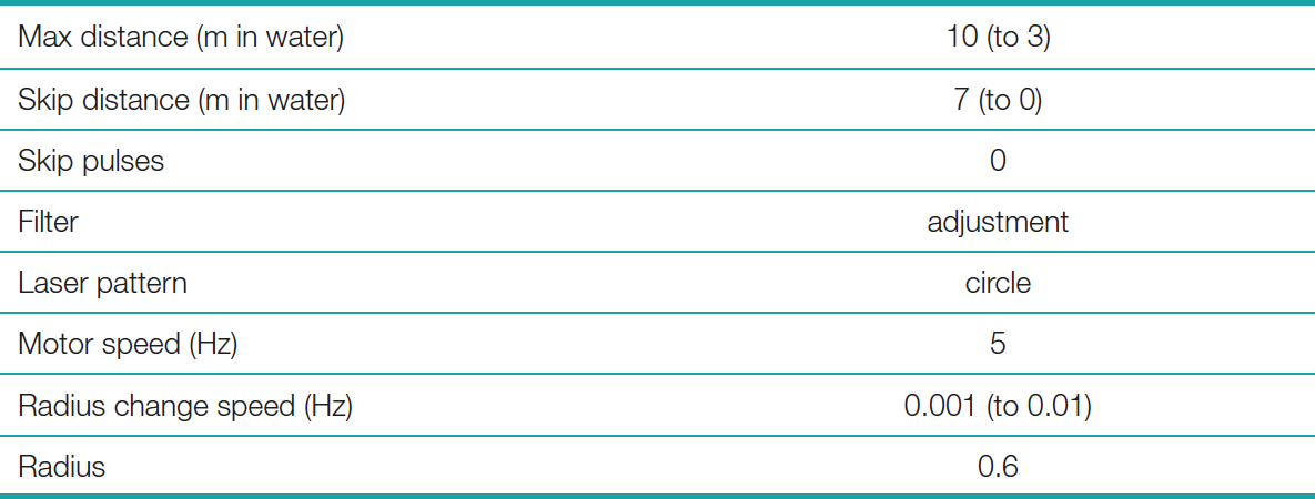
To acquire the data, the settings summarized in the following Table 2, were used. To determine the resolution of the underwater laser scanner, the Böhler star was positioned in varying distances. Subsequently, the distance between the lenses of ULi and the front panel of the Böhler star reached from a maximum of 8.03 m down to 1.03 m. To minimize the occurrence of noise, caused by reflections from the side walls as well as from the floor of the basin, the parameters “maximum distance” and “skip distance” were adapted. This limitation of recorded data in a specific range drastically decreased the final file size. To enhance the eye safety around the glass basin, the filter level “adjustment” was selected. Subsequently, the green laser did not operate at full power, but was emitted with a strength corresponding to the lowest possible laser class 2M. All other specified parameters are given in the Table 2.
To assess how the distance between the front and the rear panel of the Böhler star would influence the overall resolution of the retrieved point cloud, three scenarios were tested. First, the panels had a maximum distance of 24.90 cm. With this panel distance, the Böhler star was placed in a distance of 8.03 m, 7.03 m, 6.03 m, 5.03 m, 4.03 m, 3.03 m, 2.03 m, 1.53 m and 1.03 m from the lenses of the underwater laser scanner. In the second and third scenario, the panel distance was reduced to 12.50 cm and 1.16 cm respectively and the Böhler star was again scanned in all nine distances.
5.2.4 Results from MUM TUHH Lab
While the waveforms were processed in Pulsalyzer, the retrieved point clouds were further evaluated in CloudCompare. Here, it becomes evident, that a decreasing distance between the front and the rear panel of the Böhler star causes an overall lower scattering of the point cloud, but makes it also more difficult to separate the reflections triggered from the front and the rear panel. The case is also depicted in Fig. 6.
In Fig. 6 (left), the front and the rear panel have a distance of 24.90 cm. As it can be seen, both panels can be clearly separated from each other. While the upper blue coloured low intensity noise of the rear panel refers to reflections caused by the aluminium profiles on which the target was fixed, the remaining blue coloured reflections are caused by the edges of the front and the rear panel where only a part of the signal was reflected from the target. The edge effects do not occur uniformly, but stronger at the surrounding edges of the panels than at the cut-out Böhler star rays. Thus, the edges of the front and the rear panel cause a smearing of the signal. This behaviour is already known from terrestrial laser scanners. Hence, ranging as well as triangulation scanners both produce a variety of wrong points in the vicinity of edges. Since the laser spot cannot be focused to point size, those wrong points are inevitable (Boehler et al., 2003). The outlined effect can also be seen in Fig. 6 (middle), where the front and the rear panel have a distance of 12.50 cm. In addition to the blue coloured noise, this arrangement of the panels causes the occurrence of dark blue coloured mixed-pixels. Mixed-pixels occur whenever two objects, in this case two panels, are spatially adjacent in the range direction. Since the laser spot illuminates both surfaces, the beam cannot distinguish between both surfaces and the reflected signal is integrated (Lichti et al., 2005; Wang et al., 2016). Hence, the resulting point does not lie on either surface and the two surfaces cannot be properly resolved in the point cloud (Schmitz et al., 2020). However, since the mixed-pixels have a lower intensity than the green coloured reflections, the front and the rear panel can still be separated from each other. For a panel distance of 1.16 cm, shown in Fig. 6 (right), the mixed-pixels are more compressed and have a higher density. As a result, the front and the rear panel cannot be accurately separated from each other.
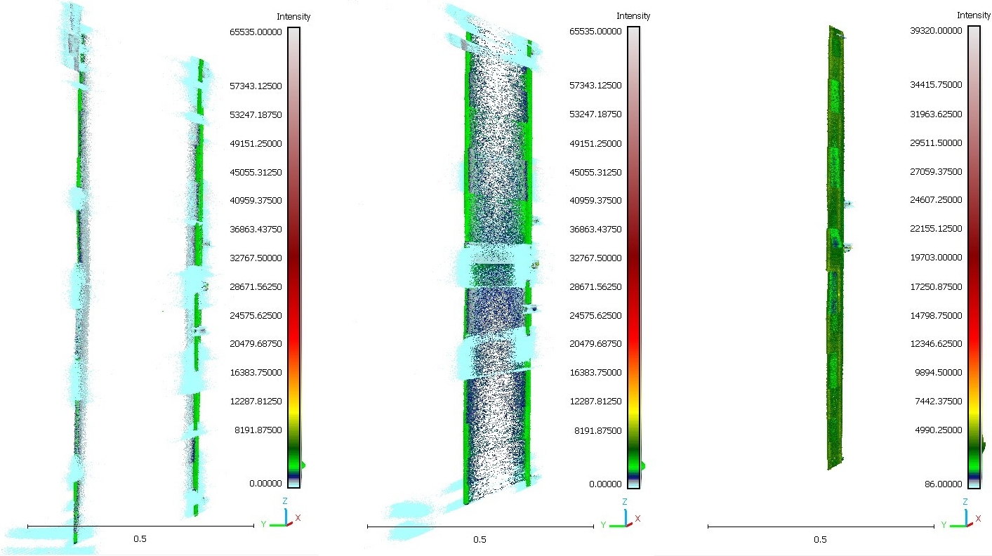
In addition to the noise caused by the edge effects and the occurrence of mixed-pixels, both panels are subject to scattering. To determine the width of the scattering for the front and for the rear panel, the point cloud was segmented. In the process of segmentation, outliers and reflections caused by edge effects were manually removed. The process of cleaning was thoroughly done by the same person and according to the same criteria. Following, a best-fit plane for the point cloud belonging to the front and the point cloud belonging to the rear panel, was computed. To numerically quantify the average deviation of the points from the fitted planes and thus gather an information about the dispersion of the point clouds relative to the plane, the root mean square error (RMSE) of the fitted planes was computed. The results are shown in Fig. 7.
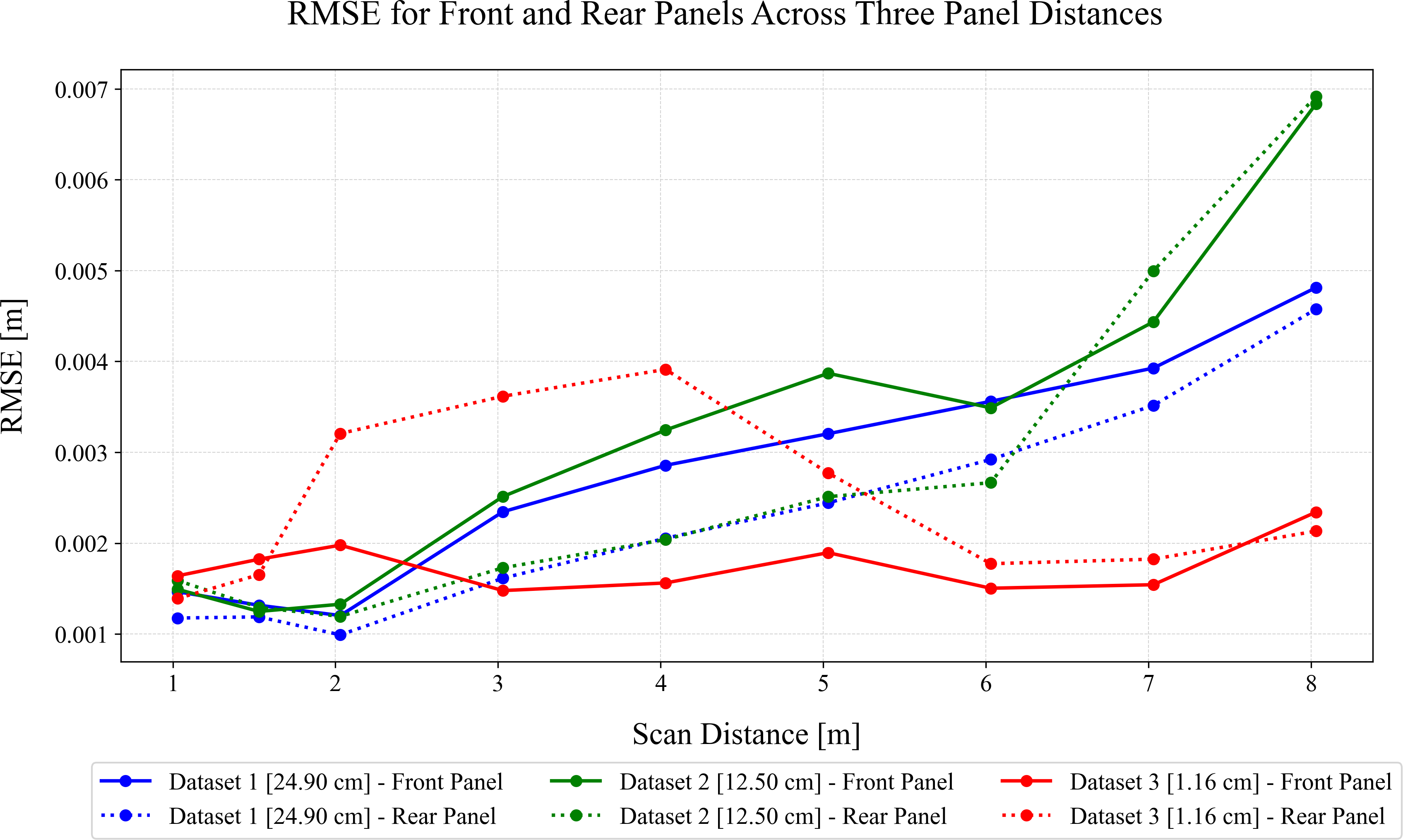
While the horizontal axis indicates the scan distance between the lenses of ULi and the front panel of the Böhler star, derived from a tape measurement, the vertical axis displays the RMSE of the fitted plane. The results for the varying panel distances, being 24.90 cm, 12.50 cm and 1.16 cm are coloured in blue, green and red respectively. While the results retrieved from the front panel are connected by a solid line, the results derived from the rear panel are connected by a dotted line.
When evaluating the first dataset, referring to a panel to panel distance of 24.90 cm, it can be seen that the overall RMSE increases with an increasing scanning distance. Subsequently, the dispersion of the point cloud increases. However, it becomes evident, that the front panel always indicates a higher dispersion than the rear panel. This behaviour applies to all scan distances. For the second data set, where the distance between the front and the rear panel was reduced to 12.50 cm, the computed RMSE for a scan distance of 1.03 m and 1.53 m is larger for the rear than for the front panel. Nevertheless, the differences are marginal and in the range of micro and nano metres. From 2.03 m to 6.03 m scanning distance, the RMSE computed for the front panel is thoroughly higher than for the rear panel. For the last two scanning distances of 7.03 m and 8.03 m, the RMSE is again larger for the rear panel than for the front panel. Subsequently, it seems that both edge cases, being a very small and a very large scanning distance, increase the dispersion on the rear panel. Nevertheless, except for the scanning distance of 5.03 m, where the RMSE difference is with 0.00136 m comparably large, the variations are overall not significant. Since the mixed-pixels were eliminated throughout the manual segmentation and thus not encountered for the plane fitting, the magnitude of the RMSE is comparable to what was derived for the first dataset. For the third dataset, where the distance between the front and the rear panel was set to 1.16 cm, the results are more or less vice-versa to the results from the second dataset. Hence, the RMSE for the two first and the last scanning distance is larger for the front than for the rear panel. For the remaining scanning distances, the behaviour changes and the computed RMSE is larger for the rear panel than for the front panel. Hence, small and large scanning distances increase the dispersion on the front panel. This is exactly opposite to what was observed for the second dataset. Despite of that, the RMSE difference for the front and the rear panel for the third dataset is comparably large. This becomes especially evident for a scanning distance of 4.03 m, where the difference is 0.0023 m. Since Fig. 6 (right) shows, that the third dataset has the least edge effects and an overall low amount of noise, this dataset should also have the lowest RMSE for the plane fitting. Hence, the high RMSE differences can be attributed to the manual segmentation, which was not only conducted on a visual basis, but which was due to the high density of mixed-pixels very difficult. Consequently, the results retrieved from the third dataset should be handled with care and treated with less resilience than the results retrieved from the first and the second dataset.
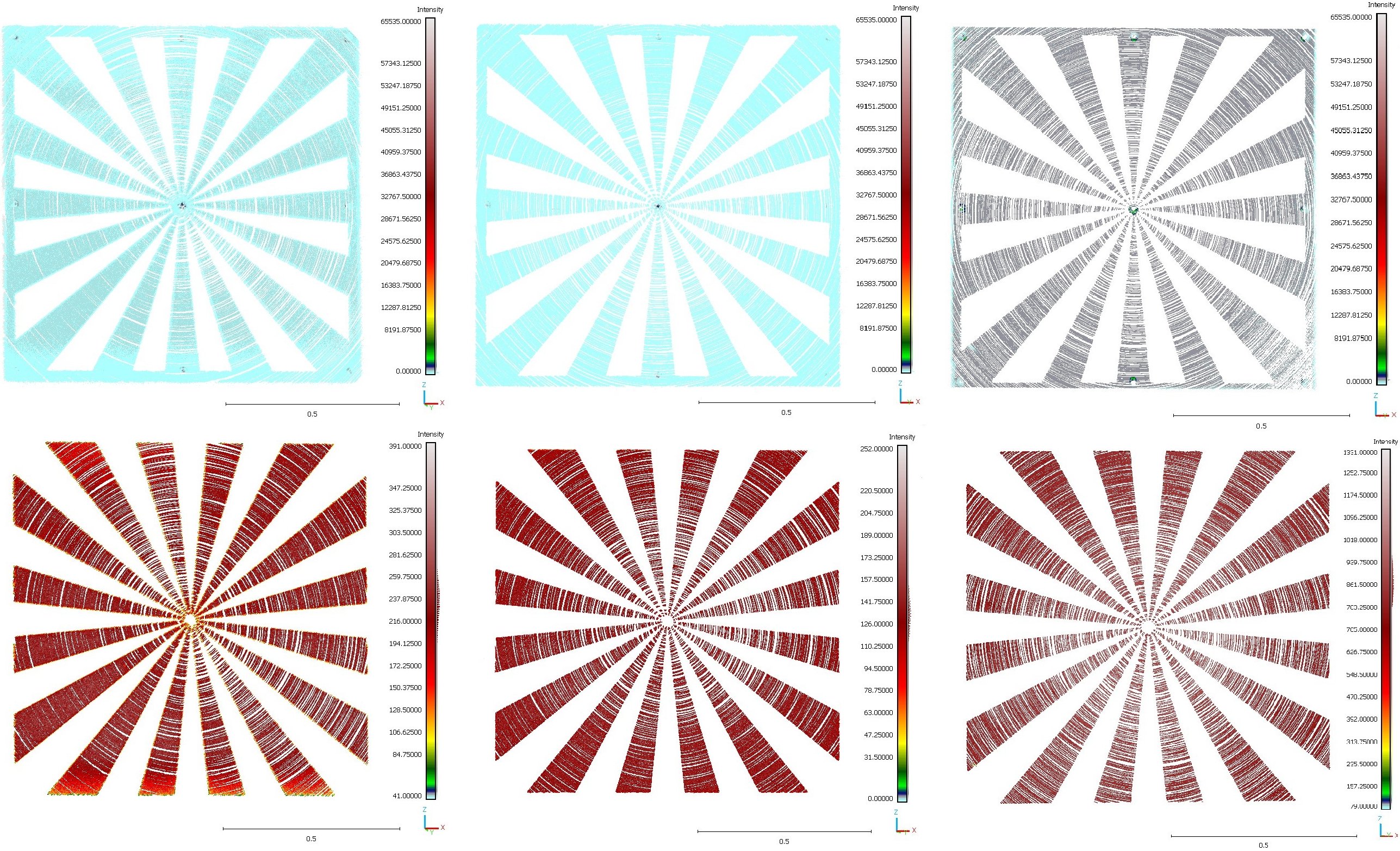
Despite the occurrence of mixed-pixels and the dispersion of the reflections triggered from the front and the rear panel, the underwater laser scanner was able to completely resolve the rays of the Böhler star. The result can be seen in the following Fig. 8. The upper three images refer to the front panel which was scanned at a distance of 8.03 m and for which the panel distance was 24.90 cm, 12.50 cm and 1.16 cm respectively. During all three scans, the centre of the Böhler star was entirely captured. The examples show, that the rays are resolved until they converge in the centre circle. Here, the length of one arc element is 2.95 mm. Similar, also the projected rays on the rear panel, illustrated by the lower three images in Fig. 8, are entirely captured until the beginning of the centre circle with a diameter of 3 cm. Equivalent results were achieved with decreasing scanning distances. Subsequently, neither the distance between the two panels nor the scanning distance itself significantly influence the depictability of the Böhler star. Following, ULi offers a very high resolution, which is primarily driven by small angular increments and a narrow laser spot size. Since the Böhler star is fully resolved in all tested configurations, another structure with more fine details to fully evaluate the performance of ULi, would be required.
5.3 Dynamic real-world close-range measurements
To evaluate the close-range performance of ULi under real-world conditions, the underwater laser scanner was mounted on the survey vessel DVocean and various measurements in a side channel of the River Elbe were carried out.
5.3.1 Integration of ULi on the survey vessel DVocean
Before the data could be acquired, several preliminary steps, including a mounting on the survey vessel DVocean, an integration into the existing network, the establishment of a time synchronization and the conduction of a calibration, were necessary.
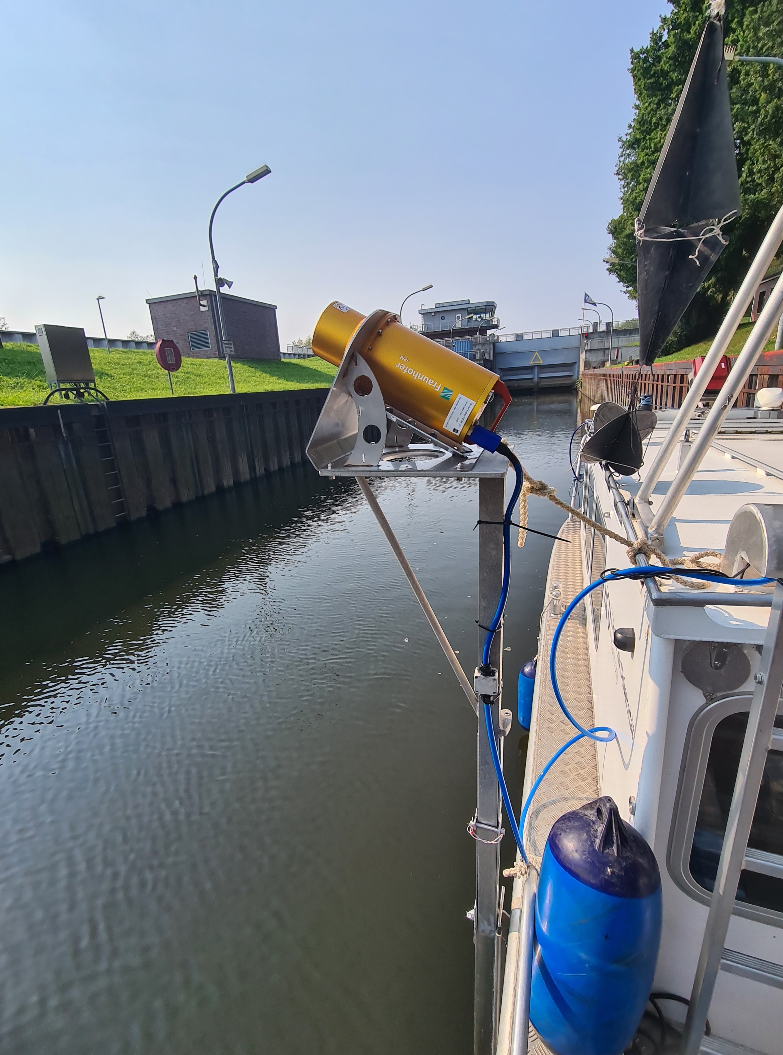
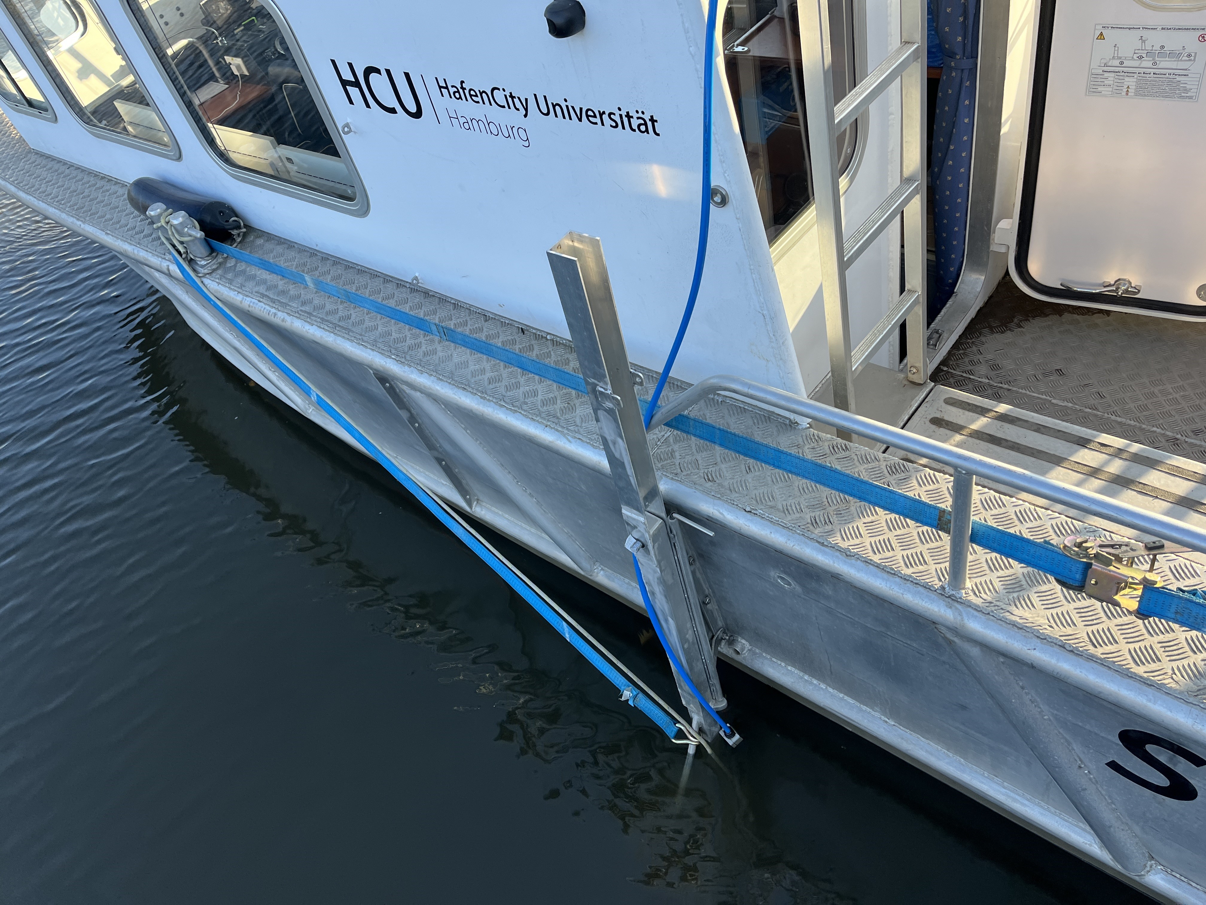
The in-house survey vessel of HCU, the DVocean, has a length of 8.00 m, a width of 2.55 m and a height above the waterline of 2.80 m. To simultaneously collect data from different sensors, the DVocean features three mounting poles – one at the bow and one on each aft side of the vessel. To accurately capture reflections from infrastructure elements such as bridge foundations or quay walls, ULi was mounted on the port-side pole. To facilitate a flexible mounting and demounting procedure, the Fraunhofer IPM designed a frame, which is also depicted in the Fig. 9a and which can be easily screwed onto the plate of the pole. A quick deployment and retrieval of ULi was achieved by folding down the pole with a leash. To minimize the movement and the vibrations of the pole in the water, caused by environmental factors such as currents, the sensor was stabilized using tensioning straps, which can also be seen in the Fig. 9b.
To integrate the scanner into the existing network on board of the DVocean, a fixed IP address and port were assigned to ULi. The processing unit was connected via ethernet to the main switch of the ship network. Therewith, the collected data could not only be directly reviewed on the screen, but they could also be combined with the trajectory information derived from the motion and position sensors on board.
To time-synchronise ULi with the trajectory recording sensors on board, a Precision Time Protocol (PTP) server, utilizing the Pulse Per Second (PPS) signal from the GNSS U-Blox evaluation kit EVK-M8T, was set up on a Raspberry 5. Since PTP hardware timestamping takes the time delay caused by the transmission of messages into account, it provides a more accurate time information in comparison to PTP software timestamping or a Network Time Protocol (NTP). To feed the PTP signal into the network, a Linux running time server on the Raspberry Pi was used. Overall, the PTP hardware timestamping resulted in a mean error and thus in an accuracy of -7.5 ns at ULi.
5.3.2 Calibration of ULi
To calibrate ULi, the position of the housing within the coordinate system of the vessel was determined. Therefore, pre-defined fix points with known coordinates, which are distributed across the vessel, were used. Equipped with a magnetic adapter and a spherical mounted reflector, those fixed based adapter points served as known reference points. To achieve the highest possible accuracy, the known fixed points were measured with a laser tracker from Hexagon. Furthermore, the housing of ULi was geometrically captured with a high-precision hand-held laser tracker from Hexagon. With the help of the 3D transformation parameters, determined from the known fixed points, the reference coordinates from ULi were transformed into the coordinate system of the vessel. A more detailed elaboration of the calibration procedure can be derived from Scheider et al. (2025).
5.3.3 Test environment Elbe
The survey was conducted on 25.10.2024 in the Tiefstackkanal in Hamburg. One key advantage of this location is that a lock separates it from the main channel of the River Elbe, which results in an overall lower sediment and salinity influx. Hence, the location offers clearer water conditions with less turbidity. To numerically verify the turbidity levels, the oceanographic profiler and a Secchi disk were used. While the probe measured a turbidity of 6.00 NTU, the Secchi depth was recorded at 1.10 m. In comparison, measurements taken in the main channel of the River Elbe showed an average turbidity of 8.60 NTU and a Secchi depth of 0.79 m, which confirmed a higher clarity of the water within the Tiefstackkanal.
5.3.4 Targets Elbe
To particular investigate the performance of ULi with regard to IMR operations and monitoring tasks, a survey along several mooring dolphins, a laying brage and two bridge foundations was conducted. To capture reflections, the DVocean was carefully navigated close to the respective targets. Subsequently, the distance between the underwater laser scanner and the mooring dolphins / laying brage / bridge foundations ranged from 1 m to a maximum of 3 m. Therewith, the targets were situated at a close range and mostly within twice the Secchi depth. To ensure a sufficient point density, the speed of the vessel was reduced to 2 kn and maintained throughout the survey.
5.3.5 Data acquisition in the river Elbe
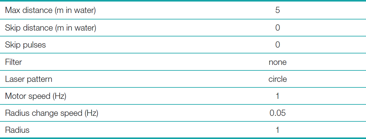
To acquire the data, the settings summarized in the following Table 3, were used. In contrast to the two laboratory measurements, the filter was set to none. Hence, the green laser operated at its maximum power, corresponding to laser class 3B.
To capture the trajectory of ULi, the raw data from the iXBlue motion sensor Hydrins – in cooperated with the Septentrio AstRx U-3 positioning system on board – was simultaneously recorded using the proprietary iXBlue software MultiLogger.
5.3.6 Results from Elbe
To process the recorded motion data and to smooth the trajectory in areas of GNSS signal outages underneath the bridge, the proprietary software Delph INS was used. Hence, a Kalman Backward- and Forward Filter was applied. The refined trajectory was exported as a text-based ASCII file which contained time, position and orientation data. This file can be imported into Pulsalyzer. However, when reviewing the processed point clouds in CloudCompare, it became evident that neither the mooring dolphins, nor the laying brage nor the bridge foundations, generated any reflection. Subsequently, the underwater laser scanner was not able to detect the targets. Given that the distance between ULi and the targets ranged from 1 m to 3 m and given that the first laboratory study revealed that ULi is able to detect close-range targets, it can be concluded that the turbidity of the water was too high. Therewith, the field test in the Elbe did not deliver any meaningful or reliable results.
6 Conclusion
The first study presented in Section 5 has shown, that the point clouds derived from the underwater laser scanner can be used to identify man-made structures such as drilled holes or cracks as well as organic structures down to a size of 2.36 mm. Nevertheless, the respective measurements exhibited a relatively high scattering up to 48 mm, which varied depending on the used material. Since the maximum distance between the lenses of the scanning unit and the target was less than 0.60 m and since the targets were not securely fixed, but only held by hand, those circumstances probably contributed to the observed high scattering. Meanwhile, the second study revealed, that a 1 m x 1 m large Böhler star is generally suitable to assess the performance of an underwater laser scanner in clear water conditions. Here, the study showed that a level-of-detail down to 2.95 mm can also be retrieved for mid-range measurements and scanning distances of up to 8.03 m. Since the Böhler star was properly fixed, the dispersion of the retrieved point clouds decreased and an overall higher quality could be achieved. Lastly, the third study, conducted under real-world conditions in a side-channel of the river Elbe did not provide any results. Subsequently, it can be said that ULi is not suitable for the operation in water bodies with a turbidity of ≥ 6 NTU or a Secchi depth of ≤ 1.10 m.
Conclusively, it can be said that a static operation of ULi generally allows to resolve structures down to the range of millimetres at close- and mid-range under controlled laboratory circumstances with a turbidity level of 0.00 NTU. Under respective water conditions, ULi is able to detect small-scale damages as cracks and holes down to a size of 2.36 mm. However, since a turbidity level of 0.00 NTU can only be achieved in laboratory environments, the usage of ULi for IMR operations as well as monitoring tasks in real-world environments, is not yet approved.
7 Outlook
To verify the statement of the manufacturer, saying that measurements carried out in clear water offer a sub-millimetre precision, further measurements in laboratory environments with advanced targets, are required. In addition, the retrieved point clouds should be compared with sophisticated ground truth measurements. Therefore, targets should be scanned with a laser tracker before they are submerged into the water. Besides, the laboratory investigations can be extended by using different scanner settings such as the line scan or other incidence angles to get a broader analysis about the resolution capability of ULi. Furthermore, the performance of ULi under even longer scanning distances should be investigated. Following, also dynamic scenarios, should be evaluated. Subsequently, it must be assessed whether a level-of-detail in the range of millimetres or even sub-millimetres can be achieved when not only the underwater laser scanner, but also the targets are moving. For this purpose, possibilities to track the respective trajectories, must be developed. Moreover, the level of turbidity at which the usage of ULi is still feasible, must be further narrowed down. On that account, laboratory environments in which the turbidity level can be precisely steered, are required. Alternatively, further tests in real water bodies, which offer lower levels of turbidity, should be conducted. Respective scenarios could involve measurement campaigns in lakes or natural sea environments with a Secchi depth of more than 2 m. Further tests in the river Elbe are, if at all, only meaningful in spring when less rainfall and a lower amount of leaves decrease the turbidity level. To further evaluate the overall performance of ULi and its suitability for IMR tasks and monitoring solutions, direct comparisons with traditional acoustic instruments, such as a multibeam echosounder or a side-scan-sonar, should be carried out.
Acknowledgements
We would like to thank the head of the HCU model workshop Sven Friedrich for processing the Resopal panels as well as Prof. Dr. Seifried and Dr. Pick from the Institute of Mechanics and Ocean Engineering of the TUHH for providing their test basin for the static laboratory mid-range measurements.
References
3D At Depth (2025). Technology – 3D at Depth are developers of the world’s first truly deepwater LiDAR. 3D at Depth Inc., Huston, USA. https://3datdepth.com/technology/ (last accessed 7 March 2025).
Alsakar, Y. M., Sakr, N. A., El-Sappagh, S., Abuhmed, T. and Elmogy, M. (2024). Underwater image restoration and enhancement: a comprehensive review of recent trends, challenges, and applications. Vis Comput, 41, 3735–3783. https://doi.org/10.1007/s00371-024-03630-w
AML Oceanographic (2025). Why choose AML for dredging applications.… AML Oceanographic Ltd., Victoria BC, Canada. https://amloceanographic.com/oceanographic-instrument-configuration-packages/aml-3-with-svp-turbidity-for-dredging (last accessed 7 March 2025).
Bianco, G., Gallo, A., Bruno, F. and Muzzupappa, M. (2011). A comparison between active and passive techniques for underwater 3D applications. The International Archives of the Photogrammetry, Remote Sensing and Spatial Information Sciences. XXXVIII-5/W16, pp. 357–363. https://doi.org/10.5194/isprsarchives-XXXVIII-5-W16-357-2011 (last accessed 1 May 2025).
Boehler, W., Bordas Vicent, M. and Marbs, A. (2003). Investigating Laser Scanner Accuracy. Proceedings of the XIXth CIPA Symposium, Antalya, Turkey. https://www.cipaheritagedocumentation.org/wp-content/uploads/2018/11/Boehler-e.a.-Investigating-laser-scanner-accuracy.pdf (last accessed 7 March 2025).
Calantropio, A. and Chiabrando, F. (2024). Underwater Cultural Heritage Documentation Using Photogrammetry. Journal of Marine Science and Engineering, 12(3), p. 413. https://doi.org/10.3390/jmse12030413
Fraunhofer IPM (2024). Underwater LiDAR System. Optical inspection of underwater infrastructure. Long range, high precision 3D mapping. Fraunhofer Institute for Physical Measurement Techniques IPM , Freiburg, Germany. https://www.ipm.fraunhofer.de/content/dam/ipm/en/PDFs/product-information/OF/AUS/Underwater-LiDAR-ULi.pdf (last accessed 7 March 2025).
Fraunhofer IPM (2025). Inspecting underwater infrastructure. Underwater Infrastructure. 3D acquisition and monitoring of large underwater structures using LiDAR. Fraunhofer Institute for Physical Measurement Techniques IPM , Freiburg, Germany. https://www.ipm.fraunhofer.de/en/bu/object-shape-detection/applications/underwater-laserscanning/underwater-laserscanning.html (last accessed 7 March 2025).
Hildebrandt, M., Kerdels, J., Albiez, J. and Kirchner, F. (2008). A practical underwater 3D-Laserscanner. OCEANS 2008, Quebec City, QC, Canada, 2008, pp. 1–5, https://doi.org/10.1109/OCEANS.2008.5151964
Hydro International. (2024). FGI harnesses Fraunhofer’s Lidar tech for maritime surveys. Geomares, Lemmers, The Netherlands. https://www.hydro-international.com/content/news/fgi-harnesses-fraunhofer-s-lidar-tech-for-maritime-surveys (last accessed 7 March 2025).
Lee, Y.-H., Kim, J.-H., Lee, S.-H. and Kim, S.-B. (2021). Underwater Excavation Records Using Underwater Acoustic Survey: A Case Study in South Korea. Applied Sciences, 11(9), 4252. https://doi.org/10.3390/app11094252
Lekkerkerk, H.-J. and Theijs, M.-J. (2011). Handbook of Offshore Surveying (Volume III, 2nd ed.). Skilltrade BV. ISBN: 978-90-816591-3-0.
Lichti, D., Gordon, S. and Tipdecho, T. (2005). Error models and propagation in directly georeferenced terrestrial laser scanner networks. Journal of Surveying Engineering, 131(4), pp. 135–142.
McLeod, D., Jacobson, J., Hardy, M. and Embry, C. (2013). Autonomous inspection using an underwater 3D LiDAR. OCEANS 2013, San Diego, pp. 1–8. https://doi.org/10.23919/OCEANS.2013.6741175
Muhammad, F. (2024). Simultaneous Underwater Vision based Mapping and Navigation [Doctoral Dissertation]. Institut Teknologi Bandung.
Nauert, F. and Kampmann, P. (2023). Inspection and maintenance of industrial infrastructure with autonomous underwater robots. Frontier in Robotic and AI, 10. https://doi.org/10.3389/frobt.2023.1240276
Ottaviano, E., Testa, A., Rea, P., Saccucci, M., Pelliccio, A. and Ruggiu, M. (2024). Experimental Activity with a Rover for Underwater Inspection. Actuators, 14(1), p. 7. https://doi.org/10.3390/act14010007
Scheider, A., Walter, A. L., Heffner, E. and Sternberg, H. (2025). Future challenge in the calibration of high-resolution hydrographic multi-sensor systems. FIG Working Week 2025, Melbourne, Australia.
Schmitz, B., Kuhlmann, H. and Holst, C. (2020). Investigating the resolution capability of terrestrial laser scanners and its impact on the effective number of measurements. ISPRS Journal of Photogrammetry and Remote Sensing, 159, pp. 41–52. https://doi.org/10.1016/j.isprsjprs.2019.11.002
Shan, J. and Toth, C. K. (2018). Topographic Laser Ranging and Scanning. Principles and Processing (2nd ed.). CRC Press.
Sun, K., Cui, W. and Chen, C. (2021). Review of Underwater Sensing Technologies and Applications. Sensors, 21(23). https://doi.org/10.3390/s21237849
Vosselman, G. and Maas, H.-G. (2010). Airborne and Terrestrial Laser Scanning. Whittles Publishing Ltd. Scotland.
Walter, A. L., Heffner, E., Scheider, A. and Sternberg, H. (2025): Underwater Laser Scanning: Integration and Testing in different environments. FIG Working Week 2025, Melbourne, Australia.
Wang, Q., Sohn, H. and Cheng, J. C. (2016). Development of a mixed pixel filter for improved dimension estimation using AMWC laser scanner. ISPRS Journal of Photogrammetry and Remote Sensing, 119, pp. 246–258. https://doi.org/10.1016/j.isprsjprs.2016.06.004
Wang, M., Zhang, K., Wei, H., Chen, W. and Zhao, T. (2024). Underwater image quality optimization: Researches, challenges, and future trends. Image and Vision Computing, 146. https://doi.org/10.1016/j.imavis.2024.104995
Witte, B. and Sparla, P. (2015). Vermessungskunde und Grundlagen der Statistik für das Bauwesen. Wichmann Verlag. Berlin, p. 208.
Zhang, S., Zhu, Y., Xiong, W., Rong, X. and Zhang, J. (2024). Bridge substructure feature extraction based on the underwater sonar point cloud data. Ocean Engineering, 294. https://doi.org/10.1016/j.oceaneng.2024.116770
Zünd (2023). Instruction Manual (Volume 1). S3 M-800. S300M081210. Product Description, p. 36.