
Abstract
1. INTRODUCTION
Traditional approaches to mapping remote, shallow waters are often expensive and challenging. In 2018 a combination of satellite, aircraft and vessel based sensors were used to survey and map the seafloor in the Ha’apai island group in the Kingdom of Tonga, an area last mapped in the late 1800’s using leadline and sextant. The latest surveys were undertaken for Toitū Te Whenua Land Information New Zealand (LINZ) in partnership with New Zealand’s Ministry of Foreign Affairs and Trade (MFAT) as part of the New Zealand Aid Programme Pacific Regional Navigation Initiative (PRNI). LINZ is the New Zealand agency responsible for producing and maintaining official nautical charts for New Zealand and a number of pacific island countries including Tonga, the Cook Islands, Niue, Samoa and Tokelau. LINZ contracted survey companies iXblue, Geomatics Data Solutions (now Woolpert Inc.) and EOMAP to undertake the work in Tonga.
Recent developments in Satellite-Derived Bathymetry (SDB) provided a way to map these remote shallow water areas with some confidence1. Combined with Airborne Laser Bathymetry (ALB) and multi-beam echo sounder (MBES) technology, it was possible to sequence data collection using SDB, ALB then MBES. This novel approach enabled LINZ and the contractors to review and refine the extent of subsequent data acquisition phases, ensuring greater efficiency and an effective survey campaign.
This article outlines the approach taken by LINZ and the contracted survey companies in conducting a successful multi-sensor survey. The article then looks at the ways the technologies were assessed and how datasets were combined for use in charting products. Finally, some recommendations are made on how the multi-sensor approach to survey can be improved.
2. SAFE SHIPPING IN THE SW PACIFIC
In 2012, in partnership with MFAT, LINZ completed a novel approach to hydrographic risk assessment2 of the Tonga region. Using GIS to build a multi-layered risk model, the approach identified shipping routes at risk, in relation to traffic type, size, density as well as volume of passengers, and compared it against a number of consequence criteria. The resulting heat-maps indicate the location and level of risk. These were then used in 2016 as the basis of discussions with Tonga to identify and prioritise a hydrographic survey programme.
The Tonga archipelago comprises 169 islands scattered over an area of 700,000 km2, stretching approximately 800km north to south. The region typically comprises clear water, fringing reefs and subsea volcanoes.


It is only relatively recently that some of the charts for Tonga have been modernised and produced in terms of WGS84 and depths in metres. A number of small scale charts were modernised in the early 1990’s with a significant number of large scale charts remaining on undetermined datums. Even then, the charts that were modernised were compiled from previously published British Admiralty charts dating from the 1900’s and incorporated ‘new’ surveys. Of particular note are the Ha’apai Group of islands that were charted in fathoms and on an undetermined datum.

Using satellite-based vessel traffic data (Automatic Identification System or S-AIS) the hydrographic risk assessment highlighted the risks to safe navigation using such charts. The images below show the tracks of domestic shipping and recreational yachts navigating in the Ha’apai islands.


The remote location of Tonga together with the vast area of water surrounding the archipelago presented a challenge to map effectively and efficiently.
In response to this problem, LINZ took a phased approach by using SDB, ALB and MBES technologies. Specifications based on existing charts established the survey extents for each sensor. As some of the charts were on undetermined datums, LINZ understood there would be a need to adjust the survey extents to ensure data was collected in the right location. The SDB data was processed in early 2018; the ALB data was acquired mid-2018; and the MBES data was acquired in late-2018.
The first phase used SDB to provide coverage throughout the entire Tonga archipelago, to a water depth of approximately 15m with a 2m resolution bathymetric dataset. This resulted in approximately 6,000km2 of the (often challenging) shallow zone being mapped. Using the SDB dataset the fathom charts were aligned so that the islands matched the observed drying line. For greater charting confidence in higher risk areas ALB and MBES survey areas were planned in the areas ‘Eua, Nomuka, Ha’afeva, Lifuka, Tofua and Kao islands. The SDB enabled LINZ and the contractors to adjust the initial flight plan for the ALB phase. This included moving flight lines from areas of deep water to cover previously uncharted isolated reef areas identified by the SDB, to fully delineate the feature with respect to least depth, position and extent. This approach was repeated to adjust the extent of the MBES survey, based on the ALB coverage. Similarly, a number of planned MBES lines were realigned to cover features identified in the ALB or just on the edge of the ALB coverage. At the MBES planning phase, coverage commenced at the 20m contour as defined in the ALB data. This decision was based on factors such as ALB system capabilities (maximum planned depth penetration), charting requirements and budget constraints.
The images below show the progression of assessing the coverage, aligning the chart to the SDB data, and the coverage achieved by the ALB and MBES. The final image shows the combined ALB and MBES coverage over and around Nomuka.

In order for SDB and ALB to be accurately depicted on charting products the two respective technologies needed to be understood. Two crucial pieces of information were needed: how accurate was the data; and, what were the feature detection capabilities of each sensor. The overlap of the datasets from the different sensors provided a good opportunity to assess the different sensors on a very large scale. As the data was applied to a wide range of product scales a more “data centric” approach was used when assessing the data.
The ALB system used for this survey was the Leica Chiroptera 4X, a shallow water system with an elliptical scan pattern. As a shallow water system the ALB was planned to capture depths to a maximum of 20m.
3. ASSESSMENT OF ALB
To assess the ALB datasets the MBES data was used as the “control” dataset. This was done as MBES has a proven track record for LINZ with its sources of error well understood and because the ALB data had been reduced to sounding datum utilising Geoid separation data, whereas the MBES used tide observations. The MBES data was gridded at a resolution of 0.5m, this was then compared to the 0.5m gridded ALB data. Both ALB and MBES datasets were gridded using the CUBE statistical algorithm which assisted comparison as limited bias had been applied in gridding. Although the ALB was specified to collect depths to 20m, depths to 35m are included in the comparisons.
As the table below indicates there is generally good vertical agreement between the ALB and MBES data. The mean difference of each dataset is within expected accuracy tolerances of the two methods and suggests that the reduction of soundings to datum is accurate. It can also be seen that the mean difference grows in areas of deeper water covered by the ALB. This is per- haps a reflection of the growing uncertainty with depth of each source dataset. In some areas the mean and standard deviation increases quickly with depth, this is particularly the case in Ha’afeva and Tofua and Kao Islands where the standard deviation doubles in the last two depth bands. The standard deviation and range of the difference is quite high, as the data was gridded at a very high resolution (0.5m) it is unlikely this can be attributed to gridding.
Tables 1, 2 and 3 : Difference comparison statistics across the different depth bands for all survey areas


It is likely the steep nature of the seabed and beam footprint size contribute to the high standard deviation and range of differences. This is supported when the assessment is repeated with high sloping areas removed, resulting in a reduction of the standard deviation and range of differences. This reduction is more pronounced in areas of steeper seabed slope such as Tofua and Kao islands
Tables 4, 5 and 6 : Difference comparison statistics across the different depth bands for all survey areas, grids with slope greater than 15° excluded


Due to the growing differences observed with depth the decision was made to exclude depths greater than 30m before merging the ALB data with the MBES data. Another consideration was the physical properties of the ALB system meant that seabed returns were intermittent beyond 30m depth. Although the above numbers would suggest that across all depths MBES and ALB agree within respective tolerances, leaving some areas of deeper ALB data in the product would result in intermittent coverage and likely create issues with later sounding selection and contour creation. It is worth noting that the inclusion of this dataset to 30m water depth exceeds the expectations of the planning phase where the ALB data was only supposed to be used in depths<20m.
4. FEATURE DETECTION
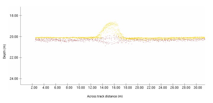
ALB data has historically been quite sparse with point spacings approximately 0.5-5m apart. The data density of the Leica Chiroptera 4X system (approx. 16pts per square metre) indicates that feature detection of a 2x2m target should theoretically be possible. During the accuracy assessment it was shown that steep features were an issue, suggesting that footprint size was a limitation in the technology. To assess the ALB feature detection capability, data was viewed against MBES data on overlapping features. Feature detection is considered demonstrated if nine returns register on the target and the height from the surrounding seabed is similar between the MBES and ALB datasets, a definition that aligns with LINZ HYSPEC3. A selection of features at different depths were investigated to understand the difference between the two systems at defining features.
Across the areas investigated some features were detected whilst others were not, examples of these are contained in the following Figures.


In some cases, the shape of the feature detected by the ALB is not as well defined as the same feature in the MBES data. More importantly the least depth is not comparable to the MBES data. This was generally observed on features in deeper water (approximately 20m).

Viewing the data across the different areas it is noticed that feature detection varied in different areas. In one of the survey areas it is noticed that feature detection is similar between the MBES and ALB across all depths. This area was Tofua and Kao Islands, two volcanic islands where a band of higher intensity seafloor reflectance can be seen around both islands.


Further investigation is required to determine why feature detection is very good in that one area and less so in others. It seems that seabed type has an influence on feature detection capabilities.
One of the limitations in the analysis was that there were not many features in depths <10m to investigate. This is a result of the MBES coverage generally commencing from the 10m water depth and so overlapping data in depths <10m was limited. Further investigation is required to determine if the ALB system accurately delineates targets in depths <10m. Another limitation is that the comparison process across all areas was manual rather than automated, which introduces a bias in the comparison. However, this approach was necessary to understand feature detection at a data centric level but adds a level of subjectivity to the results. The analysis revealed that approximately half the features sampled were not fully detected by the ALB in terms of extent and least depth. As a hydrographic authority the appetite for risk is very low and if there is any doubt in the representation of hazards on the seabed then this needs to be communicated to the mariner.
A more systematic approach could be achieved by comparing sounding selections from the different sensors (SDB, ALB and MBES). This would allow the impact to be assessed for the purpose of charting products. Of course, this approach would mean the data has only been assessed at the one scale which would mean that the assessment would need to be repeated for any larger scale products made from the data in the future. The other limitation is that coverage between the sensors should be similar and cover features across a wide range of depths. In the case of this survey, as full MBES coverage was not required in depths <10m, shoals detected by the ALB in depths <10m were not fully identified by the MBES.
Due to the variable nature of feature detection the decision was made to designate the ALB data to Category of Zones in Confidence (CATZOC) 4 B rating as opposed to an A1 rating which reflects the achieved accuracy. It is possible that feature detection is improved in critical depth areas (depths <10m) or in areas with greater seabed reflectance but it is difficult to prove with certainty. Even if that is the case it would add a level of complexity to the CATZOC information populated in the chart products if the ALB data were split into different Zones of Confidence based on depth. More understanding of the feature detection capabilities of the sensor is required before assigning a higher CATZOC to the ALB data. Ideally this would involve conducting a feature detection test over different areas of surrounding seabed, ideally at different depths. This may also guide innovation in the way the ALB data is processed to improve feature detection across different areas.

For use on the charting products the ALB CUBE surface was merged with the MBES CUBE surface. Merging with the MBES was done based on a shoal bias approach, acknowledging that both datasets were very close vertically and that the most risk averse surface was used for charting. Merging with a shoal bias was prudent with the uncertainty associated with ALB data in steep areas. In terms of the S-57 M_QUAL object for the merged dataset, the TECSOU attribute was populated with ‘found by multi-beam’ in the area where the ALB and MBES overlap.
Assessment of SDB
The overlapping MBES and ALB data acquired during the survey provided an excellent opportunity for assessment over a very large area with different characteristics such as water depth/seabed types and water clarity. As the MBES and ALB data was comparable in most areas the two CUBE surface deliverables were combined into one shoal biased grid, at 2m resolution. The SDB grid was produced at the spatial resolution of the Worldview 2/3 sensor, 2m. This meant that the two grids could be easily compared. Only vertical accuracy was assessed as unlike ALB the data density of the SDB product did not fully support feature detection, as defined by LINZ HYSPEC, i.e. a 2m resolution dataset is unable to achieve multiple returns on a 2m target.
Table 7 : Summary table of the differences of SDB to MBES/ALB surface, split by depth range

It was clear from the outset that SDB vertical accuracy decreases with depth. To understand this better the merged MBES and ALB datasets were split into discrete depth bands (0-5m, 5-10m and 10-15m). This was then compared to the SDB derived surface in two of the regions in Tonga (Nomuka and Lifuka).
Nomuka Results
As expected the differences in shallow areas are less than in deeper areas. The differences, when binned into a histogram, closely follow the shape of a bell curve indicating a normal distribution. It is also noted that the distribution is skewed to the shoaler side for all depth bands in the Nomuka area.


To further understand how accuracy can change with depth, in particular what accuracy can be obtained in depth critical areas (<2m) the data was analysed at a more granular level. The SDB data was assessed against the MBES/ALB data at increments of 2m. The results are contained in the Table below.

The results of the 2m increment are very similar to the 5m increment data and it can be seen that accuracy quickly degrades with depth. It is worth mentioning that the shape of the distribution is very similar between the 2m increment bands and the 5m increment bands, both datasets showing an increase of the distribution curve with depth.
Early in the process it was evident that the differences were greater on steep sided features (reefs/steep banks) so it was decided to exclude these areas from the analysis. This was done by calculating the slope for the MBES/ALB surface and excluding areas with a slope greater than 15°. The reason for this is that gridded datasets do not represent steep areas well, particularly at the base of the feature when dealing with a 2m grid resolution in reef areas where a depth change of 5m across a 2m horizontal grid cell is possible.

Removing the slopes from the assessment has little impact and only slightly reduces the standard deviation of the difference in two of the depth bands. It is interesting that the mean is made slightly worse, perhaps indicating the systematic shoal bias of the SDB data. Removing steep slopes however does reduce the range of differences in the dataset as one would expect.
Some small pockets of difference remain due to other environmental factors. One area of noticeable difference is on the leeward side of a small reef. In this area the SDB is significantly shallower than the MBES/ALB data. Assessing the satellite imagery, a patch of white water on the leeward side of the reef, caused by a breaking wave, is creating this large difference. Spectral properties of water would typically show white water as very shallow. Although this is a large pocket of inaccurate SDB data it looks to be an isolated occurrence in the dataset and had little impact on the depiction of the reef on the chart as it is generalised with the adjacent reef feature at the chart scale.

Some areas were identified where the SDB depths were significantly deeper than the MBES/ALB. These areas were around the edges of very shallow fringing reefs. This could be due to shading or limitations in representing the seabed as a 2m grid. Several other areas were identified where the reef/shoal was darker in colour than other sections of fringing reef. Several of these areas are shown below. The first of the areas is within a reef structure so has no significance on the charting outcome – the surrounding reefs will take precedence in most charting representations. The second area may have an impact on charting products, particularly if the area was to be represented on a larger scale chart as several isolated features were captured approximately 3-4m deeper in the SDB data than the MBES/ALB control data.


Lifuka Results
All differences in the Lifuka area showed a deep bias. The table below presents the statistics of the difference surfaces generated.

The deep bias is best illustrated by viewing a histogram plot of the differences across the surface (see Figure below). There is a significant number of differences which fall on the deep side and a noticeable “bump” in the curve on the deep side. This is quite different to the results from the Nomuka area and is a consequence of the difference between the two areas – Lifuka has a higher proportion of depth areas within the range of 5-15m. Also noticed is the same characteristic of a widening difference curve with depth, something seen in the difference statistics in the table above.
Having large areas incorrectly portrayed as too deep, even if the relative error is not large, is a concern for a charting authority, it also creates problems when merging the data with overlapping datasets.

Removing sloping areas, the differences improve slightly but the deep bias still exists. The table below presents the results of comparisons after slopes greater than 15° were removed from the surfaces.

It also seems that the differences and range of differences are similar in depths beyond 5m and that accuracy does not degrade with depth in the same way. This is different to the Nomuka area and the reason could be a result of the contrasting images of the seabed, one being darker/ rockier, but both in the depth ranges of 5-15m. The differences between the two areas can be seen in the figure below. Both areas have similar depths.

From the assessment it appears the spectral databases used for the physics based SDB approach may not be capturing subtle changes in seabed type from area to area.
It is likely that the SDB will benefit from a 2 stepped approach to processing if a multi-sensor survey is taking place. A first pass is useful for planning other sensors and detecting large shallow features (e.g. larger than 2m, the pixel size of the image data). This first pass may also be the final bathymetry data set for those areas where the other technologies are not able to be deployed, due to remoteness of location. A second step could involve checking and if necessary, re-processing the SDB based on overlapping data from the other sensors. With this second step of reprocessing it is possible that SDB coverage can be extrapolated out to a wider area with increased certainty of its accuracy.
5. DATA PORTRAYAL AND CATZOC
When incorporating the data from multi-sensors on nautical products it was necessary to consider how best to portray the data and capture CATZOC attributes for the M_QUAL object. With multiple data sources (SDB, ALB and MBES) it was important to provide the mariner with a clear picture of the data source and quality, without cluttering the chart – both ENC and paper. Producing CATZOC polygons based on technique of sounding (TECSOU), sounding accuracy (SOUACC) and water depth were not considered appropriate in this situation. A seabed comprising fringing reefs with steep topography and rapidly changing depths over short distances, would result in numerous narrow polygons.
In the case of the Tonga SDB, the decision was made to clip all SDB data to depths ≤8m. This was done primarily to remove vertical misalignment issues when merging with the ALB data. When investigating a suitable way of portraying the SDB data on chart products, LINZ considered the use of magenta polygons to define the areas. However, the Tonga charts already include magenta polygons that depict other features such as Special Management Areas and no-anchorage areas. Including another magenta polygon would increase clutter and possibly cause confusion. Instead, the SDB data is treated as another data source and included in the Source Data Diagram (below left) on the paper chart, and the TECSOU encoded as ‘satellite imagery’ on the ENC. In addition, chart notes (below right) are included with the products indicating that some depths were based on satellite imagery and could have an uncertainty of up to 3m – a figure determined by the comparisons above.

In portraying the vertical accuracy of SDB data, another consideration was to display the uncertainty as a percentage of depth. Stating that depths may have a vertical uncertainty of up to 30% of the depth may provide the mariner with more understandable information. It also acknowledges that in shallower locations (depths <5m) depths may be more accurate than the 2-3m vertical uncertainty represented by a CATZOC C rating.
6. CONCLUSIONS
A multi-sensor survey approach has many benefits. It enabled the bathymetric coverage over a very wide area with less effort than vessel-based techniques alone. The sequence of the survey enabled more effective utilisation of resources and increased vessel safety in what was a sparsely charted area. Since no mobilisation or fieldwork is required for the SDB, these data were delivered rapidly as a first phase of the project, contributing to the planning component and further optimising the overall project timelines and resources.
The different sensors performed well in the Tongan survey areas and achieved excellent coverage. The different sensors while providing the bathymetry required also acquired topographic and imagery data to support activities beyond nautical charting.
As a result of the survey 12 ENCs and 7 paper charts were updated with plans to update 4 more of each in the future. A majority of which contain data from all three sensors.
In order for the different datasets to be displayed on charting products a better understanding of the technologies was required. The results of the analysis were not simple; it is difficult to portray “good in some areas, but not so good in others”. A degree of simplification was required for placing the information on charting products.
The ALB data was very good and comparable to the MBES datasets in terms of vertical accuracy. Some uncertainty remains as to the feature detection capabilities of the ALB system for safety of navigation purposes. SDB vertical accuracy decreases rapidly with depth and therefore its uncertainty is best captured as a percentage of depth. Furthermore, SDB is at odds with the current CATZOC criteria, one that was developed with older positioning technologies in mind. Taking the new IHO survey standards as guidance, a separate CATZOC category may need to be defined for SDB, which takes into account both the relatively high horizontal accuracy as well as the depth-dependent vertical accuracy term of the SDB data.
The multi-sensor approach would benefit from a few improvements. One improvement would be to revisit and re-process some of the earlier acquired datasets using the later acquired data. For an approach like this to be adopted more overlapping data would be required in shallower areas which would provide the means to do additional processing. The area of overlap should not be a factor but the spatial distribution of overlapping areas should be a key consideration. Ideally several higher confidence MBES sites would be acquired in shallow water. Of course when planning this extra work there will be an additional cost and the benefits of the extra cost need to be taken into consideration.
Furthermore a feature detection trial involving a target of known dimensions should be conducted with the ALB sensor. Ideally this should be done in different areas and different surrounding seabed types. The logistics of this may be difficult as these need to be placed or be found with vessel resources in advance of the plane’s mobilisation. The additional trials will give more certainty of how the sensor detects features and may also guide processing efforts later in the project or in future projects.
7. REFERENCES
– 1EOMAP, Satellite Derived Bathymetry Survey Report, HYD2017/18-03 (HS60), Phase 2, 2018
– 2 MFAT, LINZ, Marico Marine NZ Ltd, South West Pacific Regional Hydrography Programme, Tonga Risk Assessment, Report Number 14NZ262-TM (https://www.linz.govt.nz/ sea/maritime-safety/improving-maritime-safety-pacific)
– 3 LINZ/NZHA, HYSPEC, Contract Specifications for Hydrographic Surveys Version 2.0 (https://www.linz.govt.nz/sea/charts/standards-and-technical-specifications-for-our-chart-and-hydrographic-work)
– 4 IHO S-57 feature object (M_QUAL) attribute, for more on S-57 see https://iho.int/en/standards-and-specifications
8. AUTHOR BIOGRAPHY
Brad Cooper completed a Bachelor of Surveying (BSurv) and IHO Cat A certification in 2011 and spent 7 years working as a hydrographic surveyor based in Perth, Australia. In this time he was involved in a number of survey projects including shallow and deep water multibeam surveys and offshore construction surveys. In 2018 he moved back to New Zealand to join LINZ as a Senior Hydrographic Surveyor. As part of this role Brad helps in the management of the HYPLAN survey programme. His responsibilities include the validation and verification of all hydrographic survey data received by LINZ for use in the production of charting products. Email: bcooper@linz.govt.nz
- EOMAP, Satellite Derived Bathymetry Survey Report, HYD2017/18-03 (HS60), Phase 2, 2018
- MFAT, LINZ, Marico Marine NZ Ltd, South West Pacific Regional Hydrography Programme, Tonga Risk Assessment, Report Number 14NZ262-TM (https://www.linz.govt.nz/sea/maritime-safety/improving-maritime-safety-pacific)
- LINZ/NZHA, HYSPEC, Contract Specifications for Hydrographic Surveys Version 2.0 (https://www.linz.govt.nz/sea/charts/standards-and-technical-specifications-for-our-chart-and-hydrographic-work)
- IHO S-57 feature object (M_QUAL) attribute, for more on S-57 see https://iho.int/en/standards-and-specifications