


Abstract
1. Introduction
Hydrographic surveyors use a wide variety of data acquisition tools and methods to collect, analyze, and characterize information about the survey area environment. These tools and methods may be quantitative in nature, such using multibeam sonar soundings to derive depths, or they may be qualitative, such as observing that a sediment sample contains brown sand.
Satellite-based optical-band (400-700 nanometers) images allow discovery and analysis of qualitative and quantitative information in areas and at scales that cannot be easily detected by the unaided human eye. The comparatively low cost and wide area coverage of satellite imagery is a valuable complement to ship-based or airborne surveys, particularly in areas with no recent data or from data of suspect quality. Repeat flyovers by satellites at regular intervals allows for change detection analysis at a given location, which is useful to determine whether a new survey is needed or whether an observed feature is real or image noise.
When analyzing optical-band satellite imagery for hydrography, there are three broad questions we can ask:
- What is the shape of the water bottom (seafloor morphology)?
- What is the thickness of the water column (bathymetry)?
- What relevant information is present and observable in the water column?
Satellite-derived bathymetry (SDB) is a quantitative image analysis method used to determine water depth – the thickness of the water column – at the time of the image. SDB analysis requires optically clear water with calm seas, minimal aerosol interference (e.g., clouds, dust), low sun-glint, and minimal surface obstructions (e.g., vessels). Water column turbidity may cause false detections or limit the utility of any individual image. As a result, images with high turbidity are typically not considered for SDB analysis regardless of the cause.
Images excluded from SDB processing due to turbidity do have value, however, as they may contain information on the seabed or water column that can be analyzed in other ways. Band analysis on multispectral satellite images is used to detect and delineate kelp beds or harmful al- gal blooms (Schroeder et al, 2019). Optical-band imagery from the RapidEye satellite has been used to evaluate temporal variation in suspended sediment concentration in rivers in Brazil (Soares et al, 2019). The presence of kelp or floating algal mats in the former and high levels of suspended sediment in the latter demonstrate the value of water column data in optical-band satellite data in aquatic environments – even though images from kelp beds in western Canada or muddy rivers in Brazil would not be considered candidates for SDB analysis.
Fugro 4DSSM is a qualitative data visualization technique that is designed to make information in a satellite image or series of images more visually intuitive to a trained human observer. It is used to assist geologists in interpreting seabed bedforms for Law of the Sea projects (van de Poll, 2004 & 2018) or other private-industry survey projects in which absolute knowledge of bathymetry is not required. Although individual scenes appear similar to a bathymetric Digital Terrain Model (DTM) or a Digital Elevation Model (DEM), Fugro 4DSSM is not a bathymetric product.
Fugro 4DSSM images are always analyzed as a time-series to determine true seafloor morphology from image noise and ephemeral data, using the principle that real seabed objects occur in the same place 100% of the time. Figure 1 shows an example of how Fugro 4DSSM is used to examine geologic features in two 4DSSM scenes based on Landsat-8 Panchromatic band images of West Caicos, Turks and Caicos, acquired 4 years apart. White arrows point to subtle bedforms that have persisted during that time, even after a direct strike in 2017 by Category V Hurricane Irma.
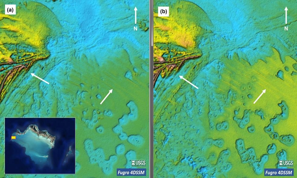
In a fortuitous finding, the authors discovered that in addition to making seabed morphology visually obvious, converting Landsat-8 source images into Fugro 4DSSM scenes made vortex structures in the water column in those images visually obvious.
Vortices are regions in a fluid in which the fluid flow rotates around a central axis. Vortex features in navigable waterways are classified according to size: mesoscale (10-200 km), sub-mesoscale (1-10 km) and microscale (10 m – 1 km). Mesoscale and larger sub-mesoscale (> 2 km) vortex features are unlikely to be found near coastlines and are unlikely to impact nearshore safety of navigation and engineering surveys.
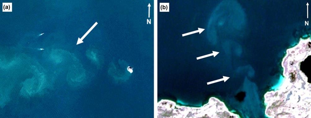
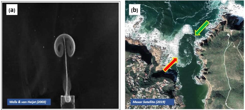
Smaller sub-mesoscale and microscale features found in navigable waterways are more likely to be of interest to hydrographers. There are two primary types of sub-mesoscale or microscale vortices observed in satellite imagery that are of interest to safety of navigation projects: Von Kármán vortex streets and vortex dipoles. Von Kármán vortex streets are a visually distinctive set of counter-rotating vortices that propagate downstream of a seabed feature and rotate inwards relative to direction of current. Vortex dipoles are counter-rotating paired vortices whose direction of rotation is away from the central axis of the source current. Figure 2 shows examples of both types of vortex patterns.
This paper examines two case studies in which sub-mesoscale and microscale vortex features are observed by inspection of optical-band imagery from Sentinel-2 and Landsat-8 satellite images: one in Saudi Arabian waters of the Arabian Gulf, and one in coastal waters of the Republic of Korea. We describe common factors leading to vortex formation and discuss how these common factors inform hydrodynamic studies and hydrographic survey planning. Finally, we make recommendations for future study of these vortex features in the context of hydrography.
Throughout this paper, qualitative information about water column vorticity is examined and analyzed in the context of necessity and sufficiency. It is necessary for an object to be a shipwreck to be classified as a hulk on a nautical chart, but not sufficient (wrecks may be fully submerged or awash). It is sufficient to be a shipwreck lying on shore to be classified as a hulk, but not necessary (hulks need not be onshore). Qualitative information that is sufficient to determine hydrographic significance helps surveyors save time, effort, and money by doing intelligent survey planning and by avoiding needless effort, especially when making decisions related to the safety of vessels and their crews. In some cases, qualitative observations are sufficient to perform chart evaluation or chart updates, such as observing during a post-hurricane survey that a fixed aid to navigation is destroyed. Although the hydrographic survey applications of observed vortex activity in both case studies are generally qualitative, they are sufficient for use in different aspects of hydrographic survey practice.
2. Methods
Source Images
Source images for both case studies are acquired by the United States Geological Survey (USGS) Landsat-8 and European Space Agency (ESA) Copernicus Sentinel-2 satellites. Publicly available source images were obtained from the USGS website https:\\earthexplorer.usgs.gov.
The Landsat-8 satellite, which occupies a near-polar orbit at a mean orbital altitude of 705 km above nominal sea level, obtains optical-band imagery from the Operational Land Imager (OLI) instrument. Radiometrically calibrated, orthorectified Level 1 Terrain Precision Correction (L1TP) images were selected to cover the entire Area of Interest (AOI) for both case studies (USGS, 2017). Band 8 (Panchromatic, 500 – 680 nm) images were used at their native 15 m resolution. Bands 2 (450 – 510 nm), 3 (530 – 590 nm), and 5 (850 – 880 nm) were used at their native 30 m resolution to create false-colour Red-Green-Blue (RGB) imagery of areas of interest.
The ESA Copernicus Sentinel-2 mission consists of two satellites, Sentinel-2A and Sentinel-2B, carrying identical payload instruments at a mean orbital altitude of 768 km above nominal sea level and operating in orbits separated by 180° (ESA, 2015). The primary imaging payload instrument is the Multi Spectral Instrument (MSI), which obtains images in 13 spectral bands. Images from both Sentinel-2A and Sentinel-2B satellites were used. Orthorectified Level-1C image tiles were selected to cover the entire AOI for both case studies. Bands 2 (central wavelength 443 nm), 3 (central wavelength 560 nm), and 4 (central wavelength 665 nm) were used to created false-colour RGB images of the AOIs. Band 3 images at their native 10 m resolution were used for Fugro 4DSSM scenes.
Source images from both satellites are georeferenced in fixed cartographic geometry using World Geodetic System of 1984 (WGS84), projected into the plane in Universal Transverse Mercator (UTM) coordinates for the appropriate longitude of the Area of Interest (AOI); this is the native georeferencing system for images from both satellites.
3. Image Selection
Image selection was performed by human users based on the following criteria:
- Presence of visible vortices in the water column
- Less than 20% total scene cloud cover
The following criteria were considered for image selection only in the context of whether vortices were visible or not:
- Water colour variations observed in RGB imagery
- Water clarity
- Sun glint
- Surface noise from wave action
- Dark-coloured seabeds (such as seagrass areas)
- Man-made surface obstructions (such as oil and gas structures or floating oyster rafts)
- Localized aerosols (such as flaring-off at offshore oil and gas structures)
- Turbulence-induced turbidity not associated with vortex activity (such as vessel wakes)
- In the Arabian Gulf AOI, aerosolized dust (as interpreted from RGB false-colour images)
In the Arabian Gulf AOI, images from the months of July and August – the summer Shamal Wind season – were excluded from consideration due to high likelihood of excess aerosols.
For Landsat-8 images, percent land cloud cover and nadir/off nadir was not considered. For Sentinel-2 images, orbit direction (ascending or descending) and satellite (Sentinel-2A or Sentinel 2-B) were not considered.
4. Image Analysis
Images for each AOI were catalogued according to satellite, date of acquisition, and time of acquisition. In the Arabian Gulf AOI, approximate phase of tide information for each image was obtained by correlating astronomical predicted tidal curves derived using the British Admiralty Simple Harmonic Method with the timestamp of the image, using the position of a single feature of interest as the benchmark location. Because this study is observational in nature, phase of tide was catalogued solely to assess variability in vortex shape over time and no attempts to compute absolute tidal height or water depths were made.
ESRI ArcGIS Pro was used for inspection and analysis of images. One map scene was created for each AOI. For simplicity, coordinate reference frames of the ArcGIS map scenes were chosen to match the native coordinate reference frames of the source images – WGS 84 UTM Zone 39 North for the Arabian Gulf AOI and WGS84 UTM Zone 52 North for the Republic of Korea AOI. Navionics Electronic Nautical Charts (ENCs) in GeoTiff format were loaded into the map scenes and converted from native coordinate reference frame into the map scene reference frame.
Red-Green-Blue false colour composite images were created using GlobalMapper software, using the band selection described previously. RGB images were then exported into GeoTiff format and added to the relevant ArcGIS map scene.
Images that were found by inspection to have good examples of different vortex morphologies were converted into Fugro 4DSSM scenes. Source images from Landsat-8 Band 8 (Panchromatic) or Sentinel-2 Band 3 images were converted to Fugro 4DSSM scenes using Blue Marble GlobalMapper and Teledyne CARIS LOTS software, using only visualization tools available in those commercial-off-the-shelf software packages (no proprietary algorithms or software add-ons are used). Because Fugro 4DSSM is solely intended to present geomorphology and water column structures in a visually intuitive manner, and is not a bathymetric product, 4DSSM images are presented without colour scales to prevent misinterpretation.
Case Study 1: Vortex Streets, Arabian Gulf, Kingdom of Saudi Arabia Study Area Background
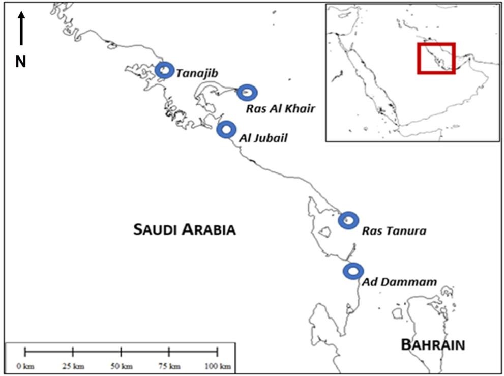
The city of Ad Dammam, Kingdom of Saudi Arabia, is home to the largest of a group of seaports serving the oil and gas industry along the Arabian Gulf coast from the Bahrain Causeway to the ports of Tanajib, Ras Saffaniyah, and R’as al Khair. (Figure 3).
Waters in this region are warm and optically clear, with a shallow shelf less than 60 m deep that ranges between 28 and 60 km from shore. Sediment type ranges from coarse to fine sand with scattered coral heads and rocky reefs occurring throughout the region. Because of the heterogeneity of seafloor features in this area, both oscillating turbulent wakes and vortex streets are present in the Arabian Gulf study area.
Von Kármán Vortex Streets
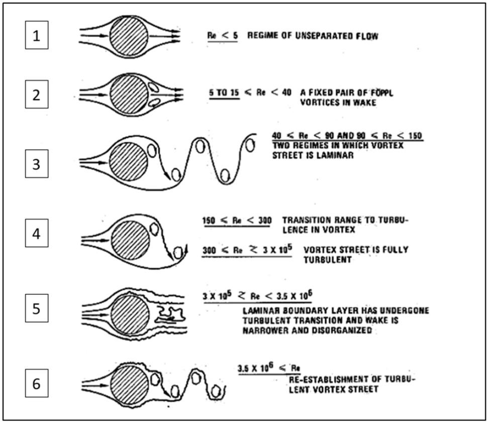
Wake flow patterns around bluff (non-streamlined) obstructions are described by the Reynolds number (Re), a dimensionless ratio of inertial forces to viscous forces within a moving fluid with different internal fluid velocities. For general cases, the Reynolds number is written as:
Equation 1.
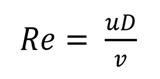
Where u is the speed of the current, D is the diameter of the bluff obstruction, and v is the kinematic viscosity of the fluid. In general, as Re increases, the wake downstream of the bluff obstruction will change as shown in Figure 4.
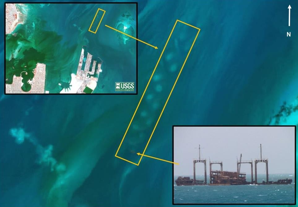
An example of a Von Kármán vortex street behind a stranded shipwreck is shown in Figure 5.
In coastal ocean environments, wakes form around islands, coral heads, shipwrecks, and other natural and anthropogenic features that are firmly fixed to (or part of) the seabed. The effects of bottom friction on the ratio between friction forces and inertial forces becomes significant, and the general-case Reynolds number must be revised to account for this. The Reynolds number for small islands (Res) is given as follows:
Equation 2.
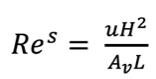
Where u is current speed, L is the cross-current diameter of the island, H is water depth, and Av is a coefficient of vertical-direction turbulent viscosity (Tomczak, 1996).
It is beyond the scope of this paper to explore methods of determining Av. It is sufficient to recognize that both current speed and water depth are significant factors in vortex street formation, and that observing a vortex street in sea water is sufficient to confirm the existence of a seabed feature.
Vortex street morphology as a function of submergence
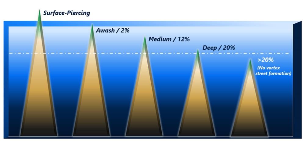
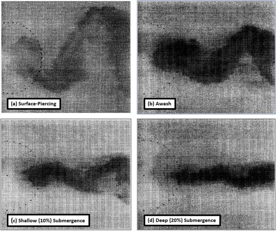
Lloyd and Stansby (1997a, b) used experimental models to demonstrate that a causal relationship exists between the shape of vortex streets behind seabed features and the submergence of the body, where submergence is defined as the ratio of flow depth H to object height h. Their model generated turbulent wakes using simulated conic islands or seamounts in water flumes at different submergence values from surface-piercing (H/h < 1.00 to H/h = 1.20). Figure 6 is a onceptual diagram that depicts relative submergence of a conical island.
Turbulent wakes were observed by injecting dye into the water flow up-current of the simulated islands/pinnacles. Observations were used to populate 2D and 3D numerical model simulations. In all experimental runs and model simulations, as submergence increased, the strength of vortex shedding decreased and the distance from bluff obstruction to the first shed vortex increased. Eventually, vortex activity disappeared entirely as water was able to flow over the top of the model bluff obstructions. Figure 7 (a-d) shows surface current vector fields of model islands at different levels of submergence.
Vortex streets at different submergence levels in the Arabian Gulf study area
Numerous vortex streets downstream of bluff obstructions are present in a single Landsat-8 OLI image dated 21 February 2019. Fortuitously, this image was acquired near low tide, and multiple vortex streets with different morphologies are observed to form downstream of seabed features.
Using the Navionics Electronic Nautical Chart (ENC) of the area to estimate feature and seabed depths and calculate submergence ratios H/h, we compare observed vortex street morphology with the experimental presentation of turbulent vortex wakes described by Lloyd and Stansby (1997 a, b) as illustrated in Figure 7. Using these comparisons, we demonstrate that vortex street presence and morphology is sufficient to make a qualitative assessment of nautical chart accuracy. Note that here, “obstruction” refers to “obstruction to flow” and does not imply that a feature is an obstruction as used in nautical chart notation.
Surface Piercing Vortex Pattern
An example of a Von Kármán vortex street can be observed in the approach to the port of Ad Dammam (See Figure 3 for location), propagating down-current from an exposed charted hulk measuring 140 m in length and 18 m beam at approximate position 26 ° 33’ 32” N, 50° 12’ 27” E. The relative position of the wreck is shown in Figure 8a and charted notation in Figure 8b.
In the Lloyd and Stansby (1997 a) surface-piercing model (or H/h = 1.00), vortex shedding begins immediately downstream of the obstruction and the wake width at the first shed vortex is greater than the diameter of the obstruction (Figure 8d). The measured distance across the vortex street starting at the first shed vortex is 270 m, over 100 m wider than the cross-current length L of the wreck (Figure 8c), which concurs with the Lloyd and Stansby model.

Awash Vortex Pattern
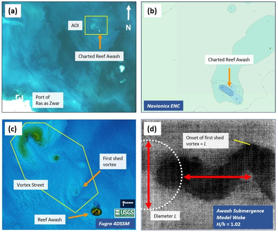
For the purposes of this paper, seabed features are defined to be awash if they are less than 1 m below the at-rest sea surface at the time of image acquisition, or if the ratio H/h ≈ 1.02.
A vortex street is observed (Figure 9a) downstream of a charted reef awash offshore of the port of Ras as Zwar (Figure 9b), located at 27° 56′ 8″ N, 49° 41′ 4″ E. The first shed vortex is approximately the characteristic diameter L downstream of the reef awash.
In the Lloyd and Stansby (1997 b) awash case, (or H/h value of 1.02) modeled oscillation of the wake begins down-current of the obstruction (Figure 9d) and distance between least depth of the obstruction and onset of the first shed vortex is approximately equal to the cross-current diameter L. Again, this real-life example has fit well with modeled awash submergence wake cases and is sufficient to confirm that the reef is properly positioned and represented on the ENC.
Mid-Submergence Pattern
In the area of Ra’s Tanaqib, Saudi Arabia (see Figure 3 for location), a charted coral head located at 28° 7′ 21″ N, 49° 10′ 13″ E (Figure 10a) has a least depth of 3m in depths of about 21 m (Figure 10b). A 4DSSM image of the area (Figure 10c) shows that the vortex morphology at this shoaling feature is defined by an oscillating wake down-current of the coral head before the first shed of the vortex street.
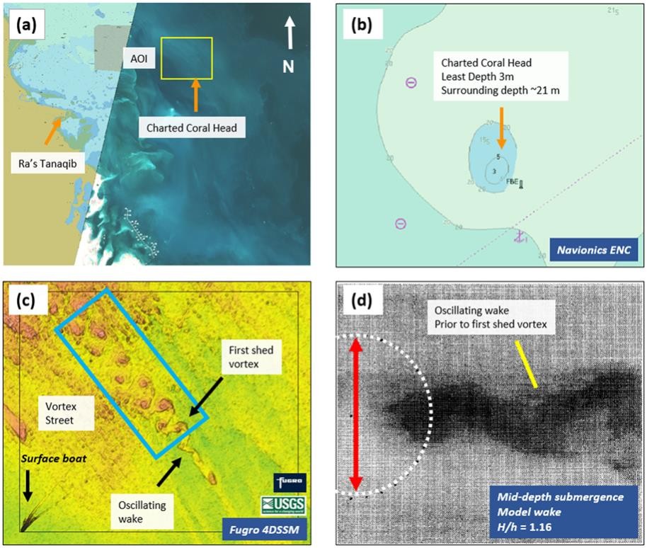
This agrees well with the modeled Lloyd and Stansby (1997 b) mid-depth submergence case (submergence ratios 1.10 < H/h < 1.16), which also shows an oscillating wake prior to vortex for- mation. If a wake of this type is observed in satellite imagery in a location where an obstruction is not charted, the hydrographer can report the that a shallowly submerged feature is probable at that location.
Deep Submergence Pattern
An vortex street typical of deep submergence was observed on a seabed feature just outside an uncharted area east of Ra’s Tanaqib at 27° 56′ 15″ N, 49° 17′ 25″ E (Figure 11). The area of interest in the Landsat-8 image (Figure 11a) corresponds to a navigational danger shown on the ENC as a navigational obstruction reported in 2003, least depth unknown (Figure 11b). Water depths in nearby areas with prior surveys are reported to be on the order of 15-18 m.
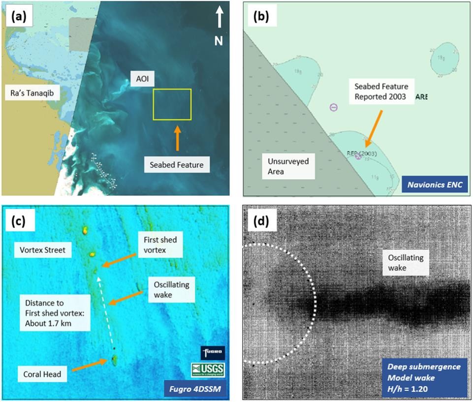
The Fugro 4DSSM scene of the feature shows a distinct coral head (Figure 11c) with a trailing vortex wake where onset of vortex shedding is 1.7 km downstream. In the deep submergence case model (submergence ratios 1.16 < H/h <1.20), water preferentially flows over the top of the obstruction rather than separating horizontally, suppressing the onset of vortex shedding. A narrow oscillating wake forms behind the obstruction and gradually changes to a weak vortex street (Lloyd and Stansby, 1997 b).
Using Vortex Street Morphology in Hydrographic Survey Practice
The existence of a vortex street seen in the water column of satellite imagery is sufficient to demonstrate that a seabed object is real, and the shape of the vortex street allows the hydrographer to quickly estimate relative least depth. Together, these are useful tools for assessing the survey area for hazards and to check chart accuracy and adequacy.
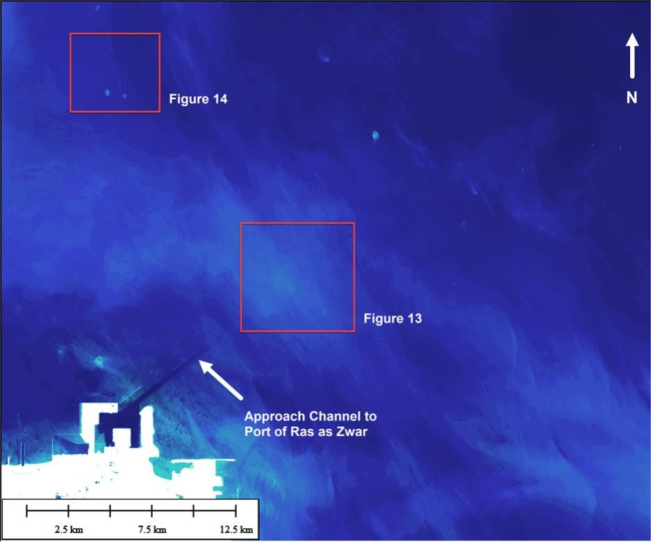
In the vicinity of the port of Ras as Zwar are two examples of how to apply this information. Figure 12 shows the general location of two inadequately charted hazards relative to the port.
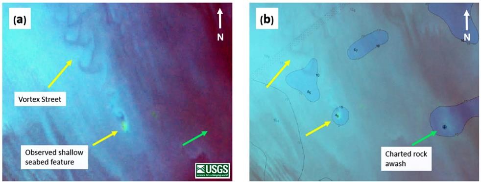
In Figure 13, a vortex street is observed flowing downstream of a coral head near the entrance channel to the port of Ras as Zwar, at 27° 37′ 22″ N, 49° 19′ 28″ E. The shape of the vortex street (Figure 13a) closely resembles an awash or shallowly-submerged object with submergence 1.02 < H/h <1.05 as per Lloyd and Stansby (1997 b). The charted least depth at the position of this coral head is 4.9 m in surrounding depths of about 10-12 m (Figure 13b), which gives a submergence value H/h = 2.04, which is too large a submergence value for a vortex street to form at all.
Green arrows in Figure 13 (a-b) point to the position of a charted rock awash. No vortex street is observed downstream of this charted rock. It is unknown if other physical factors prohibiting vortex street formation are present (vortex streets are sufficient for hazard identification, but not necessary). This charted rock awash is approximately 3.2 km east of the uncharted dangerous rock identified by the vortex street. It is unknown if the charted rock awash is incorrectly positioned on the ENC or if two rocks exist.
The presence of the vortex street is sufficient to conclude that a real feature exists at that point, that the charted least depth at that position is incorrect, and to flag the both the newly found rock and existing charted rock as requiring further surveying. A prudent hydrographer may use this information to issue a Notice to Mariners warning of a dangerous rock with least depth unknown to ensure that mariners approaching the Ras as Zwar channel can give the hazard wide clearance. This information is also suitable for survey planning, particularly in planning safe operations around a dangerous rock of unknown depth for a vessel-based survey.
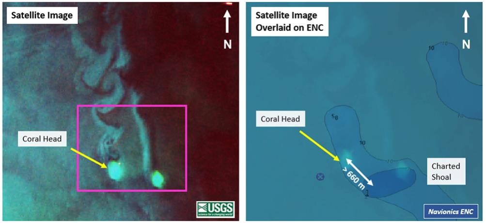
A second example of using vortex wakes to resolve low-certainty position and depth is shown in Figure 14. A pair of charted coral heads with turbulent wakes, located at 27° 44’2 1″ N, 49° 11′ 30″ E, are shown in a Landsat-8 imagery (Figure 14a) and the Navionics ENC for the area (Figure 14b). The western coral head has a vortex street wake that suggests that the coral head is awash or drying at low water. The eastern coral head has an oscillating bubble wake that dissipates as it encounters the vortex street.
Satellite imagery overlaid on the nautical chart shows that the distance as measured from the center of the western coral head to the center of the charted low-water area is greater than 660 m. For immediate safety to navigation, the position of the coral head can be sent out via Notice to Mariners as a dangerous rock, least depth unknown. This position can later be quantitatively updated to International Hydrographic Organization (IHO)-compliant position and least-depth accuracies using SDB or in-situ surveying.
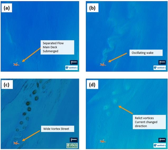
Variation in the presence and shape of vortex streets at different stages of tide is visible in imagery of the charted hulk in Ad Dammam first described in Figure 5. The shape of the wake behind the exposed hulk varies according to phase of tide (Figure 15 a-d) and illustrates the need to investigate satellite images acquired at several points through a tidal cycle. Although the superstructure and masts of the wreck are surface piercing at all phases of tide, the shape of the wake in Figure 14 (b) suggests that the main deck of the wreck is awash or shallowly submerged. Curiously, vortex streets were not observed in any images acquired during periods of rising tide, although the ephemeral relict vortices of a vortex street formed during a falling tide are visible in an image acquired one hour after low tide (Figure 15d). These relict vortices are interpreted to have sufficient residual rotational energy to persist in despite the change in tidal stream magnitude and direction.
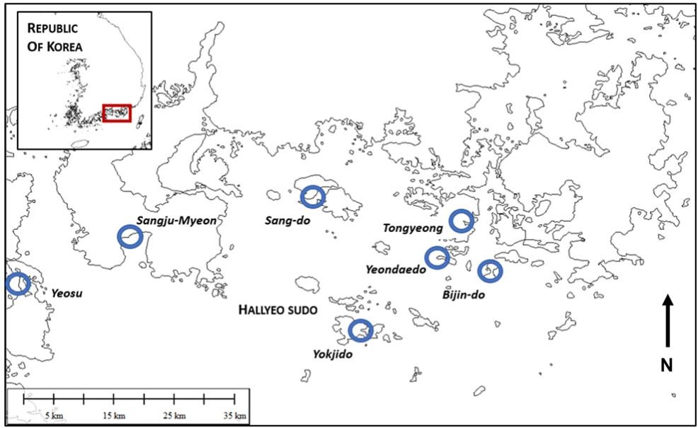
Case Study 2: Vortex Dipoles, Hallyeo Sudo, Republic of Korea Study Area Background
The Hallyeo Sudo waterway is an open bay between the Goseong Peninsula and the Yeosu Peninsula, on the east side of the Korea Strait in the Republic of Korea (Figure 16). The ports of Tongyeong, Yeosu, Geoje, and Sacheon are located on islands and peninsulas surrounding the embayment. Coves and small basins around the individual islands are home to aquaculture rafts growing oysters for consumption and for pearl production. The islands and islets vary in cross-current diameter from islets 50 m in diameter to inhabited islands more than 4 km wide, with clusters of islands separated by shallow channels less than 15 m deep. Charted water depths in open-water areas vary from 60 – 200 m.
Local sea conditions in the Hallyeo Sudo area are influenced by the presence of the East Korea Warm Current, a branch of the Kuroshio Current. With this close proximity to a fast-flowing western boundary current, Hallyeo Sudo waters are typically warm (on the order of 25 °C) and turbid with strong currents and seasonally variable salinity as Yellow Sea and East China Sea waters are entrained into the flow (Park et al, 1999). Although currents are not uniform in strength or direction across the study area, current velocities in Hallyeo Sudo are uniformly strong enough to support vortex formation.
Vortex Dipoles
When a strong, near-coastal current flows from a topographically constrained environment to an open-water, lower-current environment, such as between an island gap or around the tip of a headland, viscous boundary layers form between the jet current and the surrounding bedforms causing high-vorticity shear layers to develop in the jet. When the high-vorticity jet current emerges from the channel into a low-vorticity basin, paired counter-rotating vortices develop. These paired vortices are referred to as a vortex dipole.
The classic presentation of a vortex dipole resembles a mushroom shape where a line drawn between the centers of counter-rotating axisymmetric vortices is normal to the direction of the jet (Figure 17a). The appearance of dipoles in coastal oceans varies due to mechanism of formation (gap-forming or headland-forming), the shape of the seabed channel, phase of tide, and prevailing currents (Kashiwai, 1985). Both classically-appearing axisymmetric vortex dipoles and asymmetric vortex dipoles appear in nature (Figure 17b) and the presence of any observed dipoles should be considered during hydrographic analysis of an area.
Vortex dipoles in navigable coastal waters are classified into two types: headland-forming and gap-forming. Headland-forming vortex dipoles will form as a jet current flows past the tip of an island, headland, or similar non-surface-piercing seabed feature when bottom drag is low relative to size of the headland and tidal excursion (Signell and Geyer, 1991). These dipoles may be preceded by monopoles (single vortex) adjacent to the stronger dipole vortex. Gap-forming dipoles develop when a sufficiently strong current passes through a narrow channel between islands or a cut in a headland. Gap-forming vortex dipoles are influenced by changes in current speed and direction at the gap caused by change in tidal streams. Both headland-forming and gap-forming vortex dipoles observed in coastal waters are three-dimensional: the seabed itself is three-dimensional, as is current flow, and thus the boundary layers that form between jet current and bedforms must also be three-dimensional.
Vortex dipoles do not grow indefinitely. Gharib et al (1998) observed that for a closed channel in a laboratory with current speed U and propagation time t divided by island gap width W in a channel of constant diameter, when the value of the dimensionless ratio
Equation 3.
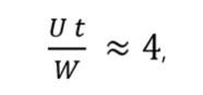
the paired vortices will separate from the jet in a process known as pinch-off. Pinched-off vortices observed in satellite imagery indicate that the jet current creating the dipoles is sufficiently strong to induce visible vorticity, even if (as is typical in tidal streams) the absolute magnitude of jet current speed varies over time. Pinched-off vortices become entrained in the prevailing currents of the low-vorticity basin.
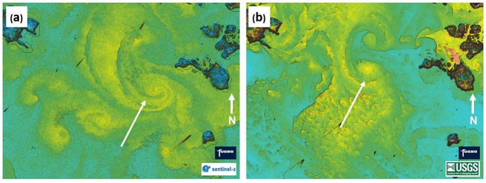
Examples of headland-forming vortex dipole are observed west of Yeondaedo Island at approximate position 34° 44’ 00” N, 128° 22′ 00″ E. The forward edge of the dipole was detected in a similar location in two Fugro 4DSSM scenes (Figure 18), however the size and symmetry of the dipole varies suggesting variability in the flow regime at the time each image was taken. For instance, on an image taken in January (Figure 18a) an asymmetric dipole form with stronger rotation in the more southerly vortex as the tidal stream passes south of the island (white arrow; Figure 18a). The appearance of an asymmetric dipole with stronger rotation in one of the two vortices is consistent with Signell and Geyer’s (1991) model where vortex growth is encouraged on one side due to low bottom drag relative to size of the headland, but vortex growth was inhibited on the other side of the headland where bottom drag was high. At a different time of year in the same area, an image taken in October (Figure 18b), shows that even though the shape of the dipole is more symmetric, the intensity of the vortex dipole is asymmetric due to drag around the headland. (Note: intensity, in this case, is interpreted by the stronger reflectivity (brighter colors) which indicates more suspended material in the water column, which in turn implies more intense rotation.)
Examples of gap-forming vortex dipoles are observed immediately north of Yokjido Island at approximate position 34° 39′ 45″ N, 128° 12′ 20″ E. A large dipole is present to west of the channel between Yokjido Island and Hanodaedo Island, and a smaller dipole is present between two islands to north and east of Yokjido island (Figure 18).
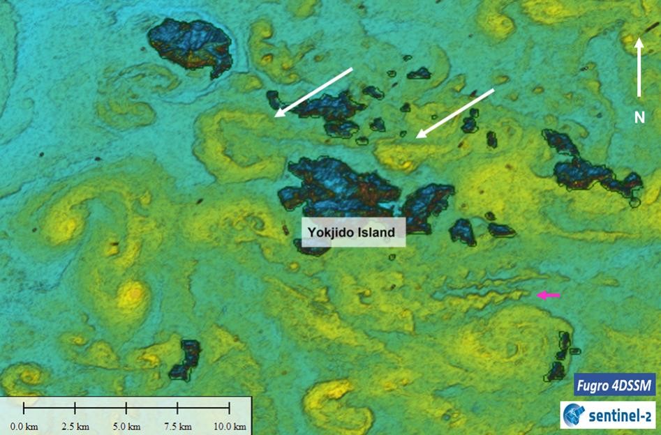
Using vortex dipoles in hydrographic survey planning
Surface currents interacting with the numerous islands of Hallyeo Sudo produce complex patterns of vortex generation. The presence of vortex dipoles is sufficient to anticipate strong currents in a hydrographic area of interest. Dipole position and orientation may be used as a proxy to estimate current speed and direction for the purposes of hydrographic survey planning. Assessing satellite imagery in this manner helps to more accurately assess operational survey needs as well as mitigating potential operational problems (such as an underpowered vessel or vehicle unable to hold line in swift currents).
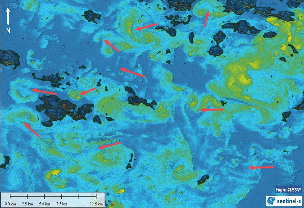
In the east of the Hallyeo Sudo, complex vortex patterns may be used to interpret the direction of surface currents (Figure 20). Red arrows indicate interpreted surface currents in the frame. A surface vessel with a multibeam echosounder running lines oblique to or across the current is likely to crab, reducing swath width and thus reducing survey efficiency. Crab angles will also reduce the position quality of towed instruments that are positioned using layback methods. By observing the positions and direction-of-propagation of vortex dipoles in several images at different phases of tide, the hydrographer may plan a more efficient, cost-effective survey.
5. Discussion
The use of water column data in optical-band satellite imagery as presented in the two case studies in this paper is novel in hydrography. There are many potential hydrographic survey uses for satellite water column data that are as yet unexplored, provided that hydrographers expand their criteria for adequate-quality satellite imagery beyond only those images that are adequate for SDB processing and seek potential uses of satellite imagery data beyond merely determining least depths for a chart.
An acknowledged limitation of this study is that it is observational and qualitative, based on remotely sensed imagery that has not been ground-truthed. Additional in-situ research with ALB or MBES is required to validate the relationship between observed morphology of vortex streets in satellite imagery and estimated submergence of the source object, and also of course to determine adequate-quality tidally reduced least depths for charting.
If it is possible to modify existing SDB algorithms or to create novel algorithms to estimate least depths for seabed features based on morphology of vortex streets, this too is suggested as a venue for additional research.
Other research topics based on this novel use of satellite imagery require both analysis of the water column itself and in-situ surveys with MBES. In-water vortex features are three-dimensional and may extend from surface to seabed. How these features interact with seabed bedforms is not well understood.
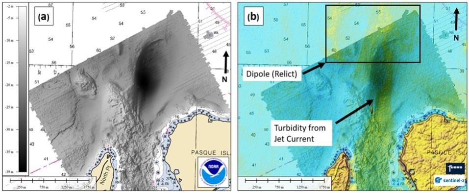
An example of where interaction between a vortex dipole and the seafloor may be studied is in Quicks Hole, Massachusetts, USA. Figure 20 (a) shows a MBES Digital Terrain Model conducted by a United States government vessel in 2004 overlaid on the corresponding NOAA raster nautical chart. In Figure 20 (b), a Fugro 4DSSM scene based on a Sentinel-2 image dated 16 March 2019 and overlaid on the NOAA bathymetry shows the presence of a vortex dipole whose maximum excursion corresponds to a large scour depression (black) in the MBES imagery. The trailing jet of the vortex dipole follows the shape of a subsea ridge observed in the MBES data. It is not known if the scour depression is a consequence of vortex dipole activity or if the collocated presence of dipole and depression is merely coincidental. Conducting additional surveys of the area with MBES water column and vessel-mounted Acoustic Doppler Current Profiler (ADCP) will shed light on this question.
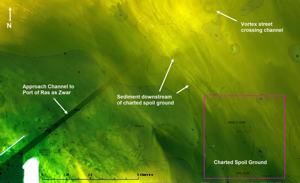
Vorticity in the water column is not the only water column data available in satellite imagery. As demonstrated by the work of Soares et al (2019) described in the Introduction to this paper, satellite imagery can be used to determine suspended sediment load. Figure 21, located in the Arabian Gulf AOI, shows the Navionics ENC of the area overlaid on false-colour imagery from the same Landsat-8 image as the case study. Suspended sediment downstream of a charted spoil ground and in the vortex street on the dangerous rock cross the dredged channel leading to the port of Ras al Khas Zwar. Combining periodic in-situ surveys of the spoil area and channel by MBES with concurrent analyses of suspended sediment load from optical-band satellite imagery is suggested to determine whether we can predict rate of shoaling or need for dredging based on time-series studies of satellite imagery.
6. Conclusions
Optical-band satellite images excluded from SDB processing due to vortex-induced turbidity have value and can add a new and useful tool into the hydrographer’s toolbox.
The authors suggest that hydrographers need not wait for further research on computational methods and may immediately begin to use imagery from available public and private satellites to review existing charts for accuracy, issue Notices to Mariners or chart updates based on findings, and plan new surveys. As computational methods become available, these too may enter the hydrographer’s toolbox.
Water column turbidity created by vortex streets and vortex dipoles that are visible in satellite imagery provides useful information about seabed morphology and water column properties such as:
- Uncharted hazards
- Depth of submerged hazards
- Local current directions
- Local current relative velocities
For best results, multiple satellite images, or time series, of the same area should be analyzed during different phases of tide, lunar months, or seasons in order to:
- Understand the hydrodynamic environment in an area
- Understanding the survey area environment as a whole, which may help with choices of equipment, line planning, and survey time constraints
- Assess chart quality for submerged hazards.
Hydrographers are encouraged to review images for vortex features and to analyze the features they find. Products may be derived from direct observation, computations, or future developments of satellite image products.
7. References
European Space Agency (2015). Sentinel-2 Data Access and Products. Retrieved from https://sentinel.esa.int/documents/247904/1848117/Sentinel-2_Data_Products_and_Access
Gharib, M., Rambod, E., and Shariff, K. (1998). “A universal time scale for vortex ring formation”, Journal of Fluid Mechanics, 360, pp. 121-140.
Kashiwai, M. (1985). “A hydraulic experiment on tidal exchange”, Journal of the Oceanographical Society of Japan, 41, pp. 11–24.
Lienhard, J. H. (1966). “Synopsis of Lift, Drag, and Vortex Frequency Data for Rigid Circular Cylinders”, Washington State University, College of Engineering, Bulletin, 300.
Lloyd, Peter and Stansby, P.K. (1997a). “Shallow-Water Flow around Model Conical Islands of Small Side Slope. I: Surface Piercing”, Journal of Hydraulic Engineering, 123(12), pp.1057-1067.
Lloyd, Peter and Stansby, P.K. (1997b). “Shallow-Water Flow around Model Conical Islands of Small Side Slope II: Surface Piercing”, Journal of Hydraulic Engineering, 123(12), pp. 1068-1077.
Marmorino, G.O., Chen, W., and Mied, R.P. (2017). “Submesoscale Tidal-Inlet Dipoles Resolved Using Stereo WorldView Imagery”, IEEE Geoscience and Remote Sensing Letters, 14, pp. 1705-1709.
O’Farrell, C., and Dabiri, J. (2014). “Pinch-off of non-axisymmetric vortex rings”, Journal of Fluid Mechanics, 740, pp. 61-96.
Park, S.-C and Yoo, Dong-Geun and Lee, Chang-Keun and Lee, Eunil. (2000). “Last glacial sea-level changes and paleogeography of the Korea (Tsushima) Strait”, Geo-Marine Letters, 20, pp. 64-71.
van de Poll, R. (2004). “Design and development of a computer-based desktop study to delimit Namibia’s continental shelf under UNCLOS Article 76 using public domain data in CARIS LOTS”, MS Thesis, University of New Brunswick, Canada.
van de Poll, R. (2018). “Using Satellite Seafloor Morphology for Coastline Delineation and Coastal Change Analysis”, Canadian Hydrographic Service, Hydrographic Remote Sensing Workshop: Ottawa, Canada
Schroeder, S.B., Dupont, C., Boyer, L., Juanes, F., and Costa, M. (2019). “Passive remote sensing technology for mapping bull kelp (Nereocystis luetkeana): A review of techniques and regional case study,” Global Ecology and Conservation, 19, e00683.
Signell, R., and Geyer, R. (1991). “Transient Eddy Formation around Headlands”. Journal of Geophysical Research, 96(C2), pp. 2561-2575
Soares Pereira, F.J., Gomes Costa, C.A., Foerster, S., Brosinsky, A., and de Araújo, J.C. (2019). “Estimation of suspended sediment concentration in an intermittent river using multi-temporal high-resolution satellite imagery.” International Journal of Applied Earth Observation and Geoinformation, 79, pp. 153-161
Tomczak, M. (1996). Shelf and Coastal Oceanography, Section 1, Chapter 7: Island wakes in deep and shallow water, Lecture Notes, http://gyre.umeoce.maine.edu/physicalocean/Tomczak/ShelfCoast/index.html
United States Geological Survey (2017). Landsat-8. United States Department of the Interior, Washington, D.C. Retrieved from https://www.usgs.gov/land-resources/nli/landsat/landsat-8?qt- science_support_page_related_con=0#
Wells, M. G., and Heijst, van, G. J. F. (2003). “A model of tidal flushing of an estuary by dipole formation”, Dynamics of Atmosphere and Oceans, 37(3), pp. 223- 244.
Williamson C. H. K. (1996). “Vortex dynamics in the cylinder wake”, Annual Review of Fluid Mechanics, 28, pp. 477-539
8. Authors Biography
Helen Stewart is an NSPS/THSOA Certified Hydrographer employed by Fugro in Houston, USA. In her broad and diverse career, Helen has worked in many different aspects of hydrography, from charting, geophysical, and deepwater AUV projects to marine construction and oceanographic research. She has a Master of Science from the University of Cape Town and a Bachelor of Science from the University of Texas at Austin. E-mail: hstewart@fugro.com
Robert van de Poll is the Global Director for Law of the Sea (LOS) at Fugro. In 1998, at the request of the United Nations, Robert developed a software suite of customized GIS tools to address all offshore Law of the Sea applications as defined in the United Nations Global UNCLOS Treaty. Robert designed, created and developed the LOS-GIS Product CARIS-LOTS. He worked at CARIS for 15 years (1991 – 2006Robert has now completed over 1800 Law of the Sea specific projects in 142 countries since joining Fugro in 2006. E-mail: rvdpoll@fugro.com
Kelley Brumley is a marine geologist and is an adjunct professor at University of Houston and Affiliate Faculty at University of Alaska Fairbanks (UAF), and a private consultant and broker on seafloor mapping projects. She received an M.S. in geology from UAF and a Ph.D. from Stanford University. Between 2006-2012, she was a member of the science party during the U.S. and Canada’s Extended Continental Shelf mapping efforts in the Arctic Ocean. Dr. Brumley has acted as lead scientist on many regional multibeam mapping and geochemical coring surveys investigating cold seep locations and related chemosynthetic habitats. E-mail: kbrumley@marietharp.org