
Abstract
1. Introduction
Most hydrographic offices (HOs) now agree that data volunteered by mariners, called variously Crowdsourced Bathymetry or (particularly in land-based applications) Volunteered Geographic Information, has potential for authoritative charting. They often disagree, however, on the extent to which it can be used, and for which purposes. NOAA, for example, has a permissive policy on “best available” data use for the chart (Office of Coast Survey, 2020), and supports the IHO Crowd-sourced Bathymetry Working Group1, hosting the IHO Data Center for Digital Bathymetry (DCDB)2 and making the data available through Amazon Web Services3. The Canadian Hydrographic Service has also used the DCDB data4 to address dangers to navigation in the Inside Passage from Seattle, WA to Juneau, AK. Other HOs have been more circumspect, often because of the difficulties posed by “uncontrolled” VBI (i.e., from any available observer), which can have unknown biases, unreliable observers, outliers, and so on. While these issues can be addressed, the cost of doing so is often considered prohibitive, and there is some question of whether a true authoritative “crowd” in the original sense (Howe, 2008) exists for bathymetry in most places (Hoy and Calder, 2019), making the term “crowd-sourced” unhelpful for discussion in this context. The term “Volunteered Bathymetric Information” is offered here as a more truthful description of the intended data source and purpose.
The difficulty is primarily that there is little pre-capture quality assurance with VBI, and a general lack of metadata. While some implementations have attempted to address installation parameters (Thornton, 2011; Van Norden and Hersey, 2012), and corrections for sound speed and other factors through oceanographic modelling has been attempted (Church, 2018), the majority of publicly available VBI does not have these refinements. Although potentially much simpler to integrate into authoritative use, more sophisticated “trusted” systems (Calder et al., 2020; Rondeau and Dion, 2020) that survey on the ellipsoid have yet to translate into scalable systems for widespread use (Desrochers et al., 2020).
Tools to assist in the assessment of VBI data are therefore required, and in particular to associate with each observer an estimate of the potential reliability, credibility, or reputation of the contributed data. Under the assumption that there is a transitive trust relationship (Severinsen et al., 2019) between the observer and the data, such a reputation metric would allow the weight of evidence associated with an observation to be assessed, allowing the HO to determine how to treat the observation for authoritative purposes. Observers with high reputation, for example, might cause a charting modification with a single observation that disagreed with the authoritative data, while less credible sources might need five, or ten, consistent observations to overturn the chart database (e.g., indicating movement of shoals). Note that this model is inclusive: authoritative observers, such as HO survey field parties, could also be assessed on the same scale, allowing their data to be tagged with “authoritative” reputation at point of creation, and then archived. This establishes a spectrum of reputation from uncontrolled VBI on one end to fully authoritative surveys on the other (Figure 1).
Reputation is not a static concept. A transitive trust relationship allows the reputation of the observer to be assessed from the observations (e.g., compared to authoritative data), but observers may change over time, initially providing poor data and improving, or forgetting to accommodate a modified configuration of the boat, and suddenly (or gradually) generating poorer data. Similarly, although data might inherit the observer’s reputation at creation time, as it ages the reputation would slowly (or rapidly, depending on the area) decay unless reinforced by new observations, until it is either contradicted by new observations, or ages out of the database. This provides a principled method for database age management.
The paper focuses on the first stage of this problem: evaluating dynamic observer reputation from archive observations, using the IHO DCDB dataset for the area of Puget Sound, WA around Seattle. Starting from the raw observations in the DCDB dataset, comparison against NOAA hydrographic datasets provides for evaluation of reputation, and estimation of vertical biases afflicting the dataset. The paper demonstrates that it is possible to evaluate a dynamic reputation estimate from observer data as outlined above.
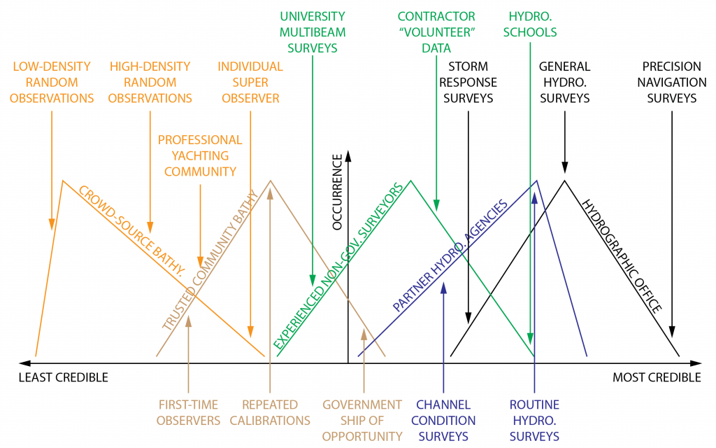
Figure 1: Notional observer reputation spectrum. The diagram shows nominal occurrence of observers against credibility for a variety of different source data types (solid lines) along with typical observers (arrows) within each color-coded population.
2. Background
There are a number of “closed garden” Volunteered Bathymetric Information (VBI) implementations: typically organized by a sonar equipment manufacturer, the users of the system contribute their observations in return for updated bathymetric products comprising the data from all users. These systems have generally focused on auxiliary bathymetric overlays, for example for fishermen or recreational boaters, which are formally adjuncts to the official charting information in the area and are often heavily interpolated, making them unsuitable for charting. The data are also usually not available outside of the system either due to data sharing limitations or the selected business model.
There are fewer systems that routinely make data available to national or international databases, and hydrographic offices (HOs) have been reluctant to use them for chart updates despite the potential and the recognition that HOs have always taken mariner reports to update the chart5, which is similar in scope. The distinction, presumably, is that previous reports were mainly from professional mariners (who knew how to report), rather than from the masses, and therefore were more limited in extent and (presumably) more likely to be plausible.
The difficulty is unreliable observers: in many cases, especially if the goal is to scale up observation, there is very limited metadata and therefore the potential for unresolved biases, and outright blunders, that would be detrimental to authoritative use. Resolving these issues is expensive: either better metadata are required, or the analyst has to attempt to evaluate each observer’s potential for providing a useful observation. The problem, then, is “assessing the credibility” of VBI (P. Wills, pers. comm.), in an automated fashion.
The subject of credibility, or more generally reputation or trustworthiness, has been the subject of much research in the general crowdsource context (Chatzopoulos et al., 2016; Whiting et al., 2017) and in the Volunteer Geographic Information, or Mobile Crowd Sensing, world (Gusmini et al., 2017; Pouryazdan et al., 2017; Severinsen et al., 2019; Truong et al., 2019), including bathymetry (Montella et al., 2019). Although the proposed solutions vary widely, they agree on some general principles. For example, that variable levels of trust or evidence are required for different applications or requestors (Severinsen et al., 2019). Or, that local observers are more valuable since they know the location and are more invested in making things better (Goodchild, 2009). And, that feedback from more reliable users is more valuable (Gusmini et al., 2017; Whiting et al., 2017) since they are more likely to be able to judge reputation of observers more accurately. The definition of reputation (or equivalent) also varies, with some researchers considering a composite of different metrics (Gusmini et al., 2017; Severinsen et al., 2019) to assess an overall “trustworthiness” for observers; Truong et al. (2019) consider, for example, a triplet model of reputation (pairwise experience between observers and data users), experience (global assessment of previous sensing), and knowledge (training, background).
There is similar general agreement on the problems to be solved for a successful system, although approaches vary in detail. Most systems assume a transitive trust model, where the data users trust the observations because they trust the observers (Severinsen et al., 2019), and allow that the reputation will vary dynamically with time so that old mistakes (or successes) do not last (Whiting et al., 2017). Many systems also focus on detection of malicious users (Chatzopolous et al., 2016; Puryazdan et al., 2017; Truong et al., 2019), which is a considerable problem in remunerated systems (i.e., where the observers are paid for their efforts), as bad actors could potentially improve their ratings to start, then feed in malicious data but still receive payments from the system. A related problem is observers who inadvertently provide bad data into the system, a more common problem with VBI systems.
The implementation of reputation assessment systems is similarly varied. All systems have some trustworthiness metric, possibly composited, although the compositing method is often ad hoc. A system must also assess the metric, either through peer review (Gusmini et al., 2017; Whiting et al., 2017) which is most commonly seen in online product reviews, or through a blended analysis with some statistical measures derived from the data (Pouryazdan et al., 2017; Truong et al., 2019). Finally, there must be a “cold start” solution (i.e., how to assign a ranking to new obser-vers). This might be simply assigning new users a generic ranking and then letting it improve through observation cycles, or to blend a prior model with observation data (Gusmini et al., 2017).
Another method is to consider paired comparisons, where there is no distinct metric to be matched, simply whether one thing is better or worse than the other. Such systems (Bradley and Terry, 1952) are often used in competitions including chess (Elo, 2008; Glickman, 1995) where player rank (essentially reputation) is computed by comparing players during a series of matches. Importantly, a more strongly ranked player essentially “donates” rank to a weaker player who defeats them, providing a mechanism for ranking to change dynamically as more comparisons are made.
This approach meets many of the requirements for a reputation ranking system, and there is a clear analogy to VBI observer reputation. Both involve comparisons between entities of different skill levels and result in a numerical estimate of skill that can be dynamically adjusted as new observations are made. This paper therefore proposes an adaptation of a pairwise ranking system originating in chess to the problem of assessing observer reputation for VBI. Observers are individually assessed using an authoritative observer (representing hydrographic archive data) as the comparison point, based on their ability to match the reference depths.
3. Methods and Data Sources
3.1. Reputation Assessment by Paired Comparison
Paired comparison systems (Bradley and Terry, 1952) are used to assess statistical significance for tests where only relative rankings of treatments are available. A common example is in taste tests where the testers rank two food preparations by preference rather than numerical scale. This process also lends itself to comparisons between game players where win/loss statistics are counted (potentially in addition to numerical scores), for example in the Elo ranking system for chess players (Elo, 2008) where the relative rank of players is computed based on win/loss records of their games against other ranked players. An extended version of this algorithm (Glickman, 1995) which includes a ranking uncertainty that can adjust for time gaps between ranking events is used here.
Consider the k th depth from the i th VBI observer, 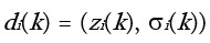 (for mean depth zi(k) with uncertatinty expressed as a standard deviation) which can be compared against the authoritative depths in the area. Each observation is equivalent to a single “game” where a “win” is declared if the depth observation matches the authoritative answer within the declared uncertainties of the observations, and a “loss” is declared otherwise. Following Glickman (1995), each observer is given a mean reputation
  and an uncertainty
  6 which reflects their ability with respect to their peers; let
  be the reputation for a single observer.
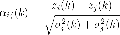
Reputations are reassessed for the VBI observers after each batch of observations. The depth agreement between observations from observers (i, j) at comparison k is
 (1)
(1)
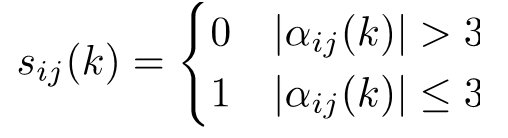
which is converted to a win (1)/loss (0) score
 (2)
(2)
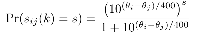
for comparison against the theoretical outcome7. For a probability model8 of
 (3)
(3)
(Bradley and Terry, 1952), Glickman (1995) shows that a Bayesian update scheme is to approximate the posterior distribution as a Normal distribution with a parameter updating scheme of 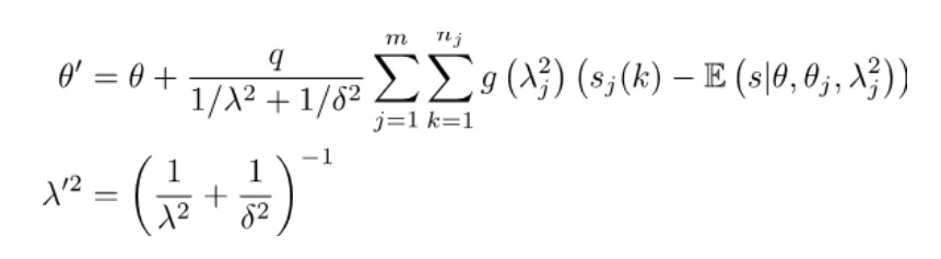 (4)
(4)
for m sources of authoritative data in the batch, each of nj comparisons (note that the dependence on the target observer, i, is suppressed for simplicity), where 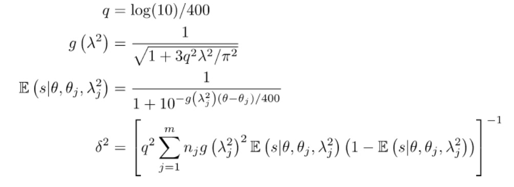 (5)
(5)
The standard expected score,  , reflects the idea that a better observer (positive difference in reputation) should be more likely to agree with the reference data, but a poorer observer will likely disagree. For bathymetric comparisons, however, there is no expectation that an observer that is not authoritative will disagree with the reference and doing so will penalize potentially good VBI observers. A modified model (Figure 2) is therefore used to express the idea that a non-authoritative observer will match the authoritative reference on average half the time, allowing potentially good new observers to gain reputation over time.
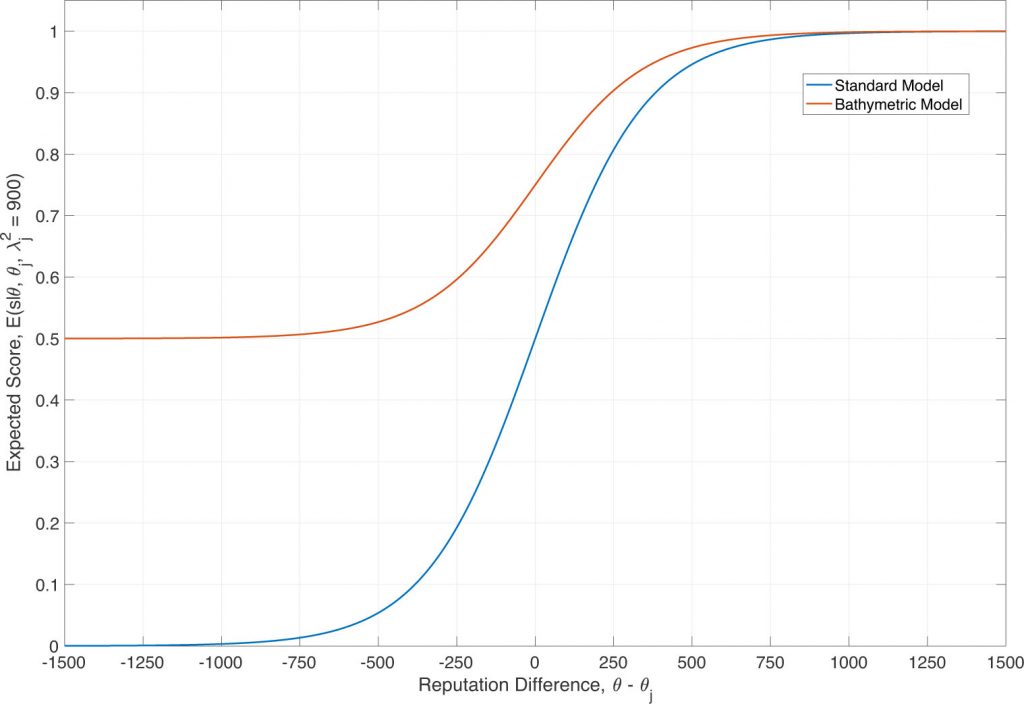
Figure 2: Expected score model. The standard model overly penalizes observers that are not authoritative (negative reputation difference)
since they are expected to disagree with the authoritative reference; the adjusted model allows for more ambivalence.
3.2. Assessment Against Authoritative Data
Each observer is initialized with a reputation of r = (1500, 350), reflecting an uninformative prior. The reputation is then updated as data are contributed, breaking the sequence of observations into 60-second batches (an observation rate of 1Hz is typical) and applying equations (4)-(5) for each batch. The second “observer” is authoritative data (processed and matched as described in Section 3.3.2), which is assumed to have a reputation equivalent to a professional surveyor (i.e., the data inherits the reputation of the observer at time of observation). In this context, rd = (2860, 30) is used (equivalent to an exceptional chess International Grandmaster), with the smaller uncertainty indicating that the reputation is well constrained.
Following Glickman (1995), the uncertainty of the reputation is adjusted for gaps in the observation sequence (e.g., between appearances of the observer in the database) to reflect the idea that a reputation is only certain if current. The uncertainty therefore grows with time duration between observation batches,
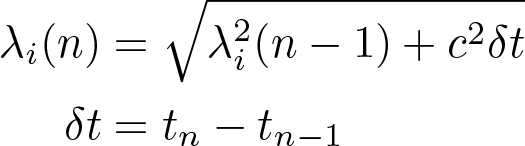 (6)
(6)
where
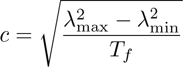 (7)
(7)
and Tf is the target time for the uncertainty to reset from minimum to maximum. In the current implementation Tf = 180 days (c = 8.752×10⁻⁶ s-1/2).
Few, if any, VBI observers have corrections applied to their data or, if they do, document what was done. Comparisons against authoritative data are therefore likely to always fail without bias assessment. Vertical correctors for water level can generally be evaluated from a nearby tide gauge or harmonic constituents, and in some instances sound speed correctors can be derived from forecast models (Church, 2018; Beaudoin et al., 2013; Lanerolle et al., 2009), or oceanographic atlases (Beaudoin et al., 2006). In smaller, or less frequented regions, however, sound speed corrections may be more difficult to obtain, and the vertical correction from the echosoun-der to the waterline is almost always missing. Consequently, an estimate of bias must be generated from the data (Section 3.3.3); this also allows the reputation assessment to distinguish between a bias of the observer and a change in the seafloor depth.
3.3. Data Sources
3.3.1. Volunteered Bathymetric Information
Data were selected from the DCDB, using only data from their “Crowd-sourced” database, which consists almost exclusively of single-beam echosounder observations from recreational mariners submitted using Rose Point Coastal Explorer through a NOAA-led pilot project. These dataconsist of any and all observations made by the volunteers, and have no outlier rejection, quality control, or other modifications from the raw observations. Although the metadata associated with DCDB records would allow the observers to record the instrumentation being used, in practice such information is rarely available, and entirely absent in the current dataset. It is assumed where necessary, therefore, that they are using conventional recreational navigational echosounders with beamwidths on order 20-30 degrees and frequencies in the range 25-200kHz, with integrated GNSS systems, potentially with differential or other WBAS augmentation.
VBI from Puget Sound in the vicinity of King County, WA (Figure 3) was selected after an examination of the data holdings because of the data density and supporting authoritative data (Section 3.3.3). A target region of (47° 27’, 47° 50’) N × (122° 09’, 122° 41’) W was selected, yielding a total of 5,599,609 possible observations. After geographic windowing to the region of interest and matching to the authoritative data (Section 3.2), a total of 1,170,261 observations remained unevenly distributed among 19 observers (Figure 4). Data were subsequently filtered to a time range of 2016-01-01 to 2019-08-10, and a depth limit of less than 11 km in order to remove clearly erroneous data; data from the same observer with duplicated timestamps were also removed. Water level corrections were then applied using the NOAA tide constituents from gauge 9447130 (Seattle, WA)9, evaluated using the PyTide10 module and applied to the data using the data’s declared time stamps as part of the pre-processing.
3.3.2. Authoritative Reference Data
NOAA-generated gridded bathymetric products, produced with multibeam echosounders (MBES) through the national hydrographic survey program, were extracted from the NOAA National Centers for Environmental Information in Bathymetric Attributed Grid (BAG) format (Calder et al., 2005), converted to ESRI ArcGrid format using a standard BAG utility, and then converted into binary MATLAB format for subsequent processing. This resulted in 22 surveys, consisting of 123 grids. NOAA hydrographic survey data sets generally consist of one or more grids of one or more resolutions, along with a low-resolution composite grid. When matching with VBI, the highest resolution grid with a valid depth at the target location was used. NOAA survey H12024 was observed to have a significant bias with respect to other observations within its lowest resolution representation (at 8m), which was removed from consideration; the report of survey (Haines, 2009) indicated difficulties with sound speed in the deepest part of Puget Sound. Only MBES data was used for this comparison in order to avoid mixing interpolation effects into the assessment (as would be inevitable with single-beam survey data). Since only a limited amount of
authoritative data is required to assess each observer, a requirement for MBES authoritative data at some location the observer inhabits is not expected to be too extreme a constraint on other implementations.
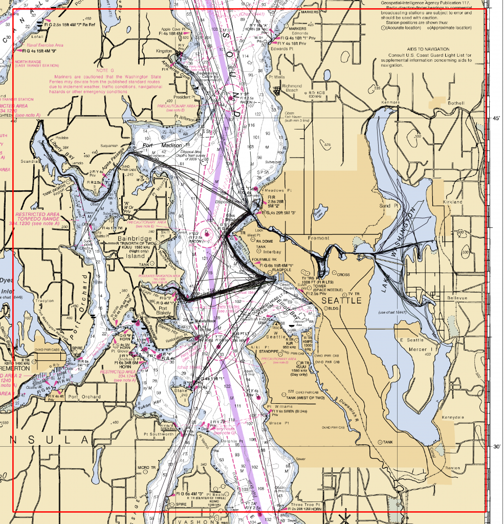
Figure 3: Data selected for experiments (area of interest in red). This represents all data available in DCDB as of 2019-07-24 for the area around Seattle, WA in southern Puget Sound.
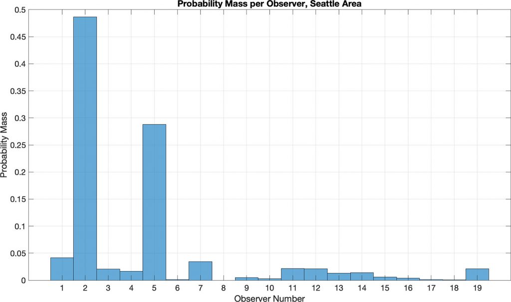
but almost half (49%) were provided by observer 2, and another ~29% by a houseboat (observer 5),
arguing against considering this a “crowd” in the conventional sense.
3.3.3. Trajectory and Bias Assessment
To facilitate analysis, each observer’s time sequence of observations was broken into transits, defined as a contiguous period of relative motion above a given speed over ground. The algorithm defined in Calder and Schwehr (2009) was used (Figure 5), with parameters Sp = 2.0 kts, Sn = 1.0 kts, T(C) = 5 min. and Tmax = 10 min. Transits of a single observation, or with position standard deviation smaller than three ship lengths were discarded as noise, or false positives.
Figure 5: Transit Determination State Machine. The algorithm starts in state “not in a transit” (¬TRANSIT), and cycles between being in a transit (TRANSIT) and checking for the end of the transit (CHECKEND) by conside-ring the current speed over ground (SOG), and whether it exceeds the start speed (Sp), and the stationary speed (Sn). The algorithm requires the “possible end of transit” to exist for at least T(C) seconds before declaring the transit complete , allowing for some drifting/idle during a transit, and limits total transit time above at Tmax to manage ships
that disappear from the record for a considerable time.
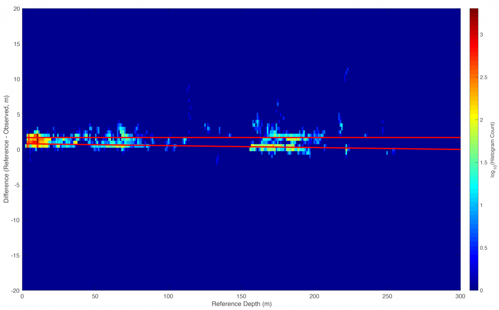
To estimate bias in each identified transit the difference between the corrected observed depth and highest resolution authoritative depth was determined, and outliers were removed by rejecting any points more than ±(5.0 + 0.05z)m from the authoritative depth z, and also in areas of significant slope where differences in depth are expected due to differences in beamwidth between consumer and survey systems. Slopes are approximated as the time differential ofauthoritative depth (and computed by first differences), with a fourth-order Butterworth IIR filter (wc = 0.1) for smoothing. Data on slopes with dz/dt > 0.15 m/s are, heuristically, removed from consideration for bias estimation (but are used otherwise). Transits with fewer than 30 observations, or with full observed depth range less than 10m, are ignored. A first order polynomial model is fit to remaining transits; models indicating bias increase of more than 10% of depth are removed.
All remaining data are then aggregated and used to compute a first-order polynomial fit for the observer. Some observers show evidence of multiple regimes (Figure 6). In this case, a preliminary inspection was used to determine breakpoints between transit groups, and to eliminate dubious transits from consideration. Separate models were then computed for each transit group.
3.3.4. Uncertainty Estimation
Uncertainty for the authoritative data is provided in the BAG files and is used directly. Static measurement uncertainty for the VBI is computed through the standard deviation of the observations for all inter-transit periods with more than 10 observations (for estimation stability), discar-ding any observations that disagree with the reference depth by more than 10%.
The effective observer uncertainty is computed from each transit by selecting windows of 120s (taking into account any time gaps), computing a first difference to remove any long-term trends, and then computing the standard deviation. Windows with fewer than 30 observations are discarded. This procedure provides a series of estimates of uncertainty that combine the basic measurement uncertainty and any residual motion effects not corrected by the observer (which is typically all motion effects in VBI), and therefore can be used directly to estimate real-time uncertainty for the system.
Water level uncertainty is estimated to include a measurement uncertainty of 0.01m, and a spatio-temporal uncertainty of 0.10m.
Overall uncertainty of corrected observations is computed by propagation of uncertainty (ISO, 1995), including effective observer uncertainty, water level uncertainty, and the estimated bias correction uncertainty based on the linear model of bias (Section 3.3.3).
4. Results
4.1. Bias Estimation
From all of the observers (Figure 4), a subset was selected based on data density (closest to 1Hz observation rate, indicating consistent data observations), and data volume (normalized by the cumulative probability density function to avoid outliers). A first run of the bias parameter algorithm was used to identify changepoints (Figure 7), after which a second run computed a final model for each group of transits. In some cases, the changepoint is not particularly obvious (Figure 8), which is likely to lead to poor corrections for depths. This is considered an extension of the estimation problem: if changes in bias are not clear, it is likely that there is significant noise in the observations, and therefore it should be considered of lower reputation.
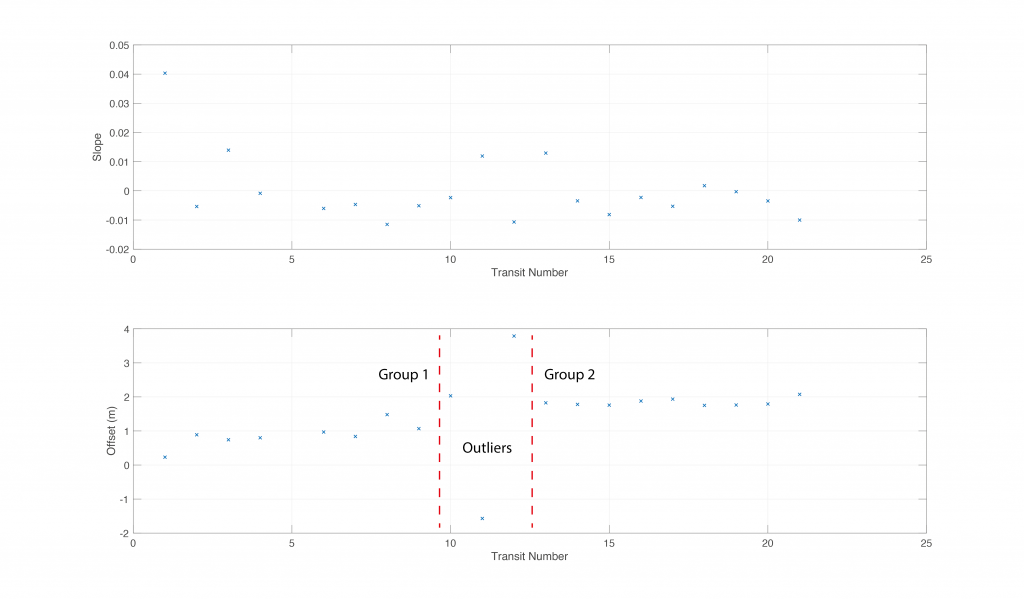
Figure 7: Example of per transit bias estimation for observer 1 (Figure 4). A clear step in linear model offset (lower panel, red dashed lines) as a function of transit number (i.e., time) shows two regimes of correction are required. The intermediate section can be classified in either regime, since the outliers are subsequently ignored.
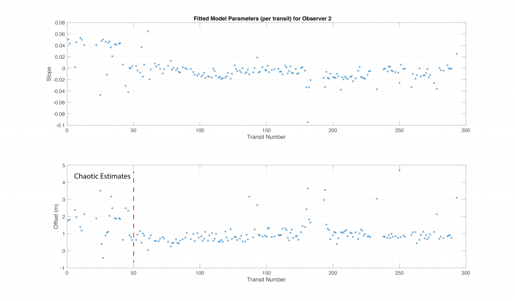
Figure 8: Example of per transit bias estimation for observer 2 (Figure 4). While there is no visually obvious changepoint in the estimates, the somewhat chaotic estimates before transit 50 (left of red dashed line) were eventually separated as a separate group; this may be noisy estimates rather than a distinct regime.
All of the observers modelled demonstrate a positive offset value, and negative slope, indicating that the observed depth is shallower than the reference depth everywhere, and increasingly so with depth, Figure 9. This reflects the effects of uncorrected sound speed in the data; correcting in this way gives an approximation, although the ability to extend these corrections elsewhere is likely to be limited (Section 5).
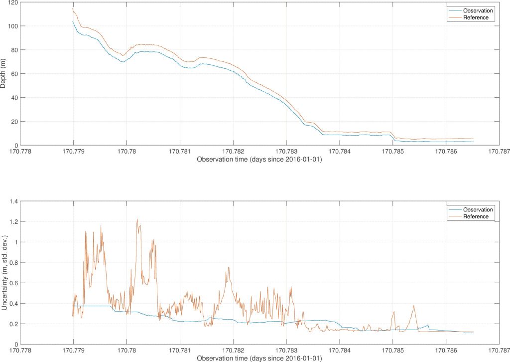
Figure 9: Pre-correction observation and reference data depth (top; note depth is positive down in this view, so vertical axis is increasing depth) and uncertainty (bottom) from observer 2. The shoal depth bias in the observation data is due to the offset between waterline and echosounder. Note 0.01 day = 1.44 min.
4.2. Reputation
Reputation assessments were generated for all transits for each observer (Section 3.2). For Observer 1, the computation indicated very reliable estimation (and bias correction), Figure 10, with the reputation rapidly increasing from the initial value to be virtually authoritative by the end of the first transit, and then continuing consistently. The reputation uncertainty also drops quickly to the minimal value and continues low due to the frequency of observations. This sort of beha-vior is indicative of an observer who could be taken seriously if even a single observation indicated a significant difference from the authoritative database, since it is likely that this really indicates a significant change in the current configuration of the seafloor.
Figure 10: Reputation estimates for the first four transits of observer 1. For four transits over ~28 hours, the observer reputation increases to almost authoritative, and then stays there; uncertainty reduces to the minimum (30) over the first few observation batches. Note 0.002 day = 2.88 min.; 0.005 day = 7.2 min.; 0.01 day = 14.4 min.
Observer 2, on the other hand, has more variable performance, Figure 11, consistent with the noisy bias estimates of Figure 8. The reputation range of ~1500 is indicative of an observer that can occasionally generate reasonable data, but which has significant outliers on occasion. For authoritative use, this would indicate that multiple observations from the same observer (or from different observers with equivalent reputation) would be required to trigger a change in charting.
After a good start, the observation quality starts to fall significantly, and the reputation drops. Note 0.005 day = 7.2 min.
Reputation is not forever, however. Later in the dataset, observer 1 goes through the transition of bias estimates observed in Figure 7 and in the process starts to disagree significantly with the reference data. The resulting reputation estimates, Figure 12, show that after agreeing with the reference data for approximately seven months, the observer starts to disagree (reputation dropping, transit 11), and then disappears from the record for approximately four months. After returning, the observer quickly re-establishes a good reputation as it heads into shallower water. The cause of this disagreement is not known, but it is tempting to interpret this as some modifications being made to the ship for an extended period of cruising, after which the modifications were removed. Another potential explanation is that the bias model changepoint was not well estimated, so that the difference reflects poor bias corrections. In either case, the reputation would provide clear evidence to an HO about the use of the observer’s data in the interim.
5. Discussion
The results here demonstrate that it is potentially possible to extract bias estimates from VBI observers, and to assess reputation, given a sufficient amount of data in an area with a reference depth dataset. Both of those caveats can be relaxed in practice: simply waiting long enough will provide sufficient data, and most observers are going to visit an area with reference depths at some point, and therefore can be calibrated for bias and reputation each time they do. Since there is no real-time requirement in VBI data, neither of these pose a limitation to practical implementation. The current corrections for sound speed are adequate since anything not corrected is reflected in the uncertainty but could be improved with model data if available (Beaudoin et al., 2006; Beaudoin et al., 2013). Motion effects in VBI, except heave, are expected to have little effect due to the wide-beam nature of most non-survey echosounders. Most VBI observers are likely to have no recordable motion estimation hardware on board in any case (except perhaps their cellphone), although it would be possible to add motion processing if these data became available. Like sound speed, uncorrected motion effects would appear in the estimated uncertainty.
The examples here assess the reputation continuously, but in practice this would limit the ability to detect changes in authoritative bathymetry (i.e., the reputation would be reduced every time an area with changed bathymetry was observed). Consequently, a functional system would need to recompute reputation at fixed intervals, or as data become available. The selection of 60-second intervals for computing reputation is arbitrary (although plausible) and could be adjusted based on experience in the field. Similarly, the choice of a six-month uncertainty reset period is arbitrary and should be adjusted depending on the number and types of ships that appear in any given dataset, and the scale of processing. For example, ships that are expected to be more stable (e.g., professionally crewed merchant mariners) might preserve their uncertainty for longer, as opposed to recreational boaters; having the processing done routinely over large areas might obviate the necessity for a detailed analysis, since boats would rarely be out of observation range. If required, Glickman (1995) provides a formal parameter estimation scheme.
The work here has focused on assessing VBI observers, but the transitive trust relationship between observers and data (Severinsen, 2019) implies that these methods could also be applied to authoritative databases. That is, each database point is imbued with the observer’s reputation at collection time, and then evolves independently as new observations are made in the same area. Confirmatory observations (from any observer) would maintain the data’s reputation; contradictory observations (from reliable observers) would reduce the reputation until the data were considered too unreliable to be useful. This method may allow for principled management of hydrographic databases, where the choice to replace or retire data is based on evidence, rather than gut feeling, or some proxy such as bathymetric uncertainty.
Apart from the processing required (which is relatively light), the suggested system makes demands of the HO, particularly that there is a willingness to set thresholds for reputation and evidence required to trigger changes to the chart. For example, how many observations from an observer with reputation (2800, 30) does it take to place a depth on the chart? How many from an observer (or set of observers) with reputation (1500, 125)? Such estimates would likely depend on the HO’s attitude towards the risk of “outside source” data, and potentially the bathymetric context of the area. Calibration from field data would likely be required.
A final potential benefit of the proposed scheme is in motivating the observers. Many Mobile Crowd Sensing (MCS) implementations rely on a perceived benefit to the observers that rewards them for their participation; often, this is a monetary payment. Such motivation is not expected for VBI, but some scheme to inform the users of their progress, particularly if it can also assist in guiding them to a better solution, is likely to be useful. The proposed scheme provides a simple estimate of “observing power” that could be readily reported to observers, and might assist with crowd retention.
6. Conclusions
This work has demonstrated that it is possible to estimate biases for Volunteered Bathymetric Information (VBI) observers, and to dynamically estimate reputation for them. Reputation is estimated on an arbitrary numeric scale and represents a measure of observer reliability since the basis is comparison against authoritative data, where available. Providing a reputation score is the first stage to a model for their use in authoritative products and methods, although such use would require further development and field calibrations by the sponsoring hydrographic office.
The methods outlined apply equally to the data made by observers, and to all observers rather than just volunteers. Doing so may allow the same methods to be used for assessment of survey adequacy and resurvey priority (through data residual reputation over time), in addition to allowing for principled ageing out of data from the database.
Acknowledgements
This research was supported by NOAA grants NA15NOS4000200 and NA20NOS4000196, and significantly benefited from the comments of the peer reviewers. The support of the Data Center for Digital Bathymetry at the NOAA National Centers for Environmental Information at Boulder in providing the data is also gratefully acknowledged.
Conflict of Interest
There are no conflicts of interest to report in this work.
7. References
– Beaudoin, J., Hughes Clarke, J.E., Bartlett, J. (2006). “Usage of Oceanographic Databases in Support of Multibeam Mapping Operations Onboard the CCGS Amundsen”, Lighthouse, 68.
– Beaudoin, J., Kelley, J.G.W., Greenlaw, J., Beduhn, T., Greenaway, S. (2013). “Oceanographic Weather Maps: Using Oceanographic Models to Improve Seabed Mapping Planning and Acquisition”, Proc. U.S. Hydro. Conf. (New Orleans, LA).
– Bradley, R.A., Terry, M.E. (1952). “Rank Analysis of Incomplete Block Designs I: The Method of Paired Comparisons”, Biometrika, 39(3/4): 324-345.
– Calder, B. R., Byrne, S., Lamey, B., Brennan, R.T., Case, J.D., Fabre, D., Gallagher, B., Ladner, R.W., Moggert, F., and Paton, M. (2005). “The Open Navigation Surface Project”, Int. Hydro. Review, 6(2) [New Series].
– Calder, B.R., Dijkstra, S.J., Hoy, S., Himschoot, K., Schofield, A. (2020). “A Design for a Trusted Community Bathymetry Systems”, Mar. Geodesy, 43(4):327-358, DOI: https://doi.org/10.1080/ 01490419.2020.1718255
– Calder, B. R. and Schwehr, K. (2009). “Traffic Analysis for the Calibration or Risk Assessment Methods”, Proc. U.S. Hydrographic Conf. (Norfolk, VA).
– Chatzopoulos, D., Ahmadi, M., Kosta, S., Hui, P. (2016). “OpenRP: A Reputation Middleware for Opportunistic Crowd Computing”, IEEE Communications Magazine, July (115-121).
– Church, I. (2018). “Linking Hydrographic Data Acquisition and Processing to Ocean Model Simulations”, Proc. Canadian Hydro. Conf., 27-29 March, Victoria, BC., Canada.
– Desrochers, J., Ndeh, D., Regular, K. (2020). “Crowd-sourced Bathymetry in Northern Canada”, Proc. Canadian Hydro. Conf., 24-27 Feb., Québec City, QC, Canada.
– Elo, A.E. (2008). “The Rating of Chess Players, Past and Present”, Ishi Press International, ISBN: 0923891277.
– Glickman, M.E. (1999). “Parameter Estimation in Large Dynamic Paired Comparison Experiments”, Appl. Statist., 48(3):377-394.
– Goodchild, M.F. (2009). “NeoGeography and the Nature of Geographic Expertise”, J. Location Based Services, 3(2):82-96.
– Gusmini, M., Jabeur, N., Karam, R., Melchiori, M., Renso, C. (2017). “Reputation Evaluation of Georeferenced Data for Crowd-sensed Applications”, Procedia Computer Science, 109C:656-663.
– Haines, D.W (2009). “Descriptive Report: Approaches to Port Madison and Shilshole Bay”, NOAA Office of Coast Survey. (https://www.ngdc.noaa.gov/nos/H12001-H14000/H12024.html).
– Howe, J. (2008). “Crowdsourcing: How the Power of the Crowd is Driving the Future of Business”, Crown Business (Random House), New York.
– Hoy, S., Calder, B.R. (2019). “The Viability of Crowdsourced Bathymetry for Authoritative Use”, Proc. U.S. Hydro. Conf. (Biloxi, MS).
– International Standards Organisation, 1995. “Guide to the Expression of Uncertainty in Measurements”, ISBN 9267101889, ISO, Geneva.
– Montella, R., Di Luccio, D., Marcellino, L., Galletti, A., Kosta, S., Giunta, G., Foster, I. (2019). “Workflow-based automatic processing for Internet of Floating Things crowdsourced data”, Future Generation Computer Systems, 94:103-119.
– Office of Coast Survey (NOAA), 2020. “Mapping U.S. Marine and Great Lakes Waters: Office of Coast Survey Contributions to a National Ocean Mapping Strategy”, NOAA Technical Report, online: https://nauticalcharts.noaa.gov/learn/docs/hydrographic-surveying/ocs-ocean-mapping-strategy.pdf [Retrieved August 24, 2020].
– Pouryazdan, M., Kantarci, B., Soyata, T., Foschini, L., Song, H. (2017). “Quantifying. User Reputation Scores, Data Trustworthiness, and User Incentives in Mobile Crowd-Sensing”, IEEE Access 5:1382-1397.
– Rondeau, M., Dion. P. (2020). “Potential of a HydroBox Crowd-sourced Bathymetric Data Logger to Support the Monitoring of the Saint-Lawrence Waterway”, Proc. Canadian Hydro. Conf., 24-27 Feb., Québec City, QC, Canada.
– Severinsen, J., de Roiste, M., Reitsma, F., Hartato, E. (2019). “VGTrust: Measuring Trust for Volunteered Geographic Information”, Int. J. GIS, 33(8):1683-1701.
– Thornton, T. (2011). “TeamSurv – Surveying with the Crowd”, Hydro. International (July/August), Lemmer, The Netherlands.
– Truong, N.B., Lee, G.M., Um, T.-W., Mackay, M. (2019). “Trust Evaluation Mechanism for User Recruitment in Mobile Crowd-Sensing in the Internet of Things”, 14(10):2705-2719.
– Van Norden, M., Hersey, J.A. (2012). “Crowdsourcing for Hydrographic Data”, Hydro. International (October), Lemmer, The Netherlands.
– Whiting, M.E., Gamage, D., Gaikwad, S.S., Gilbee, A., Goyal, S., Ballav, A., Majeti, D., Chhibber, N., Richmond-Fuller, A., Vargus, F., Sarma, T.S., Chandrakanthan, V., Moura, T., Salih, M.H., Kalejaiye, G.B.T., Ginzberg, A., Mullings, C.A., Dayan, Y., Milland, K., Orefice, H., Regino, J., Parsi, S., Mainali, K., Sehgal, V., Matin, S., Sinha, A., Vaish, R., Bernstein, M.S. (2017). “Crowd Guilds: Worked-lef Reputation and Feedback on Crowdsourcing Platforms”, Proc. CSCW 2107, Feb. 25 – March 1, Portland, OR.
8. Author Biography
Brian Calder graduated M.Eng (Merit) and Ph.D. in Electrical and Electronic Engineering from Heriot-Watt University, Scotland, in 1994 and 1997 respectively. He was a founding member of the Center for Coastal and Ocean Mapping (CCOM) & NOAA-UNH Joint Hydrographic Center at the University of New Hampshire, where he is currently Associate Director (CCOM) and a Research Professor. His research interests focus mainly on bathymetric data processing, including the estimation, use, and presentation of uncertainty; and the efficient implementation of the associated algorithms.
Email: brc@ccom.unh.edu
- https://iho.int/en/csbwg
- https://www.ngdc.noaa.gov/iho/
- https://odp-noaa-nesdis-ncei-csb-docs.s3-us-west-2.amazonaws.com/readme.htm
- https://www.nauticalcharts.noaa.gov/updates/noaa-announces-launch-of-crowdsourced-bathymetry-database/
- For example, NOAA’s reporting service, at https://www.nauticalcharts.noaa.gov/customer-service/assist/.
- The ranges here are as used in chess rankings, and are essentially arbitrary but should be considered relatively (i.e., a reputation of (2860, 35) is considerably better than one of (1200, 350) for example).
- Since
 ij (k) is a normalized z-score, this is equivalent of considering three standard deviations of the depth agreement to be significant.
 - The constant 400 here is an estimate of the reputation between players likely to cause a significant change in scores.
- https://tidesandcurrents.noaa.gov/stationhome.html?id=9447130
- https://pypi.org/project/pytides/