


Abstract
1. Introduction
1.1 The Hydrographic Health Model (HHM)
The United States of America has collected hydrographic data for charting purposes covering 3.4 million square nautical miles of coastal and continental shelf waters since the early 1800s. Collection methodologies have significantly advanced from the earliest lead-line surveys having a data density equivalent to chart sounding density, to the modern multibeam echosounder (MBES) technology collecting thousands of data points each ping (Hawley, 1931; Adams, 1942; Van Der Wal and Pye, 2003; Calder, 2006; Wong et al., 2007). The National Oceanographic and Atmospheric Administration (NOAA) is the U.S. organization responsible for the collection, management, and publication of these data and the over 1000 nautical charts to which they contribute. NOAA reports that they obtain about 3,000 square nautical miles of new coverage annually from their four survey ships and additional outsourced contract work (Gonsalves et al., 2015; Keown et al., 2016; Fandel et al., 2017; Hicks et al., 2017), making survey prioritization essential. Traditionally, this is performed by experienced hydrographers, though more recently NOAA has developed a model to identify these areas called the Hydrographic Health Model (HHM) (Keown et al., 2016; Fandel et al., 2017; Hicks et al., 2017).
The HHM is a risk-based approach to approximate the current state of charted data that relies primarily on survey quality assessments and the associated risks to those vessels with out of date soundings. While this heuristically accounts for some environmental change factors such as storms, tides, and marine debris, it could be improved with the inclusion of quantifiable and more dynamic, area-specific estimates of change. Specifically, the inclusion of hydrodynamic variables could refine the accuracy of the HHM and resultant risk factors as they drive regional and nearshore sediment transport patterns.
Presently, the HHM is implemented in ESRI ArcGIS with a 500 m resolution output and relies on the difference between the present and desired survey scores (or the hydrographic gap) to assess the quality of survey data. The core HHM equation multiplies the estimated hydrographic risk,  , by the hydrographic gap of a specific area,
  , such that,
 (1)
(1)
resulting in a nondimensional rating ranging from less than 0 to 100, with the healthiest (or most recent surveys) scoring near or below 0 to demonstrate a lack of need. The hydrographic risk is a subjective mathematical weighting function that rates consequences and likelihoods on a scale of 1-5 with 5 presenting the most risk (Keown et al., 2016; Fandel et al., 2017; Hicks et al. 2017).
The hydrographic gap of currently charted data is determined by the difference between the estimated present survey score (PSS) and a user-defined desired survey score (DSS),
 (2)
(2)
The PSS and DSS terms are populated with values (0-110) that closely correspond to the International Hydrographic Organization (IHO) categorical zone of confidence (CATZOC) level coverage specifications (IHO S-57, 2014; Keown et al., 2016; Fandel et al., 2017; Hicks et al. 2017). The DSS variable is completely user-defined and is essentially meant to delineate areas that have high accuracy requirements (like navigational channels and ports) from those that are not as stringent (like in deep water areas). The definition can be as specific or general as desired. However, NOAA’s DSS specifics are outlined in Table 1.
Table 1

The PSS is defined by  (3)
(3)
where the survey’s initial score, ζ, is depreciated by an empirical exponential decay based on the age of the survey, T, weighted by an empirical function C that depends on several changeability variables including heuristic estimates of the number of large storms, tidal currents, marine debris, and an empirical factor (Keown et al., 2016; Fandel et al., 2017). Although these variables do not always result in physical changes and their absence does not necessarily equate to a stable environment, they generally characterize areas of navigational interest with hydrographically relevant information. More objective methods to estimate the hydrographic gap (2) could include observation of bathymetric change. Additionally, local hydrodynamic variables drive sediment transport patterns that lead to erosion and deposition, and their inclusion could markedly improve the accuracy of predicted chart health estimates. However, a direct application of these estimates into the current iteration of the HHM is not presently possible.
1.2 Hydrographic Uncertainty Gap (HUG)
Our premise is that the hydrographic gap of the HHM could be modified to integrate relevant values of bathymetric change and have units expressed in meters (or normalized by the total water depth). As such, the modified gap equation proposed herein utilizes the quantification of vertical uncertainty through annually observed average rates of change to characterize the risk of inaccurate charted depths (Taylor, 1982), and it is henceforth referred to as the hydrographic uncertainty gap (HUG).
The HUG model,  , is defined as
 (4)
(4)
a measure of the difference (reported in meters) between the estimated present uncertainty, σpresent, and the maximum allowable uncertainty, σmax, each essentially taking the place of the PSS and DSS terms respectively, in the HHM. Here, σpresent incorporates temporal variability (rate of change of the seafloor) and assessments of data quality with (5)
(5)
where the temporal rate of change of the seafloor elevation, ∆z/∆t, is multiplied by a time period, ∆T, that can correspond to the survey age but can also be used to represent changes in bathmetric depths a given time frame into the future. The initial uncertainty, σinitial, is the vertical uncertainty (in meters) of a given survey at the time of collection.
In (4), the maximum allowable uncertainty in meters, σmax, is a user-defined variable based on a desired CATZOC level and derived using the associated IHO vertical uncertainty equation, (6)
(6)
where a and b are IHO S-44 order-dependent parameters (IHO S-44, 2008) and d is depth (in meters). Differencing the σpresent and σmax estimates the hydrographic uncertainty gap of a given charted region. Normalizing by d recasts the results in terms of the fraction of water depth. Positive values from this calculation indicate that the uncertainty exceeds allowable limits, while negative values indicate areas within the desired uncertainty limit. Through this methodology we expect to more robustly identify degrading regions that exceed acceptable variability as outlined by IHO survey standards.
Understanding how a given area will change in the future allows for more comprehensive resource allocation, updates to disaster response requirements, and better understanding of how climate change scenarios may impact charted waters. It is important to note that the various temporal variability estimates are not required to be used together. Instead, through this assessment, we show how to utilize publicly available data to better estimate bathymetric change, and to further outline how numerical modeling could be useful.
Given that 200 years of data have been incorporated into U.S. charts, a vast span of technologies have been used, and the unstable nature of the data acquisition environment, establishing a present and initial uncertainty estimate for all charted data could be rather complex. Here we outline a methodology for calculating the uncertainty for an entire survey area with archived data sets, constraining that uncertainty where appropriate using available vessel Automatic Identification System (AIS) data, and assess the resulting area uncertainty. When combined with the temporal variability component, an integrated assessment of the current hydrographic state of an area can be constructed.
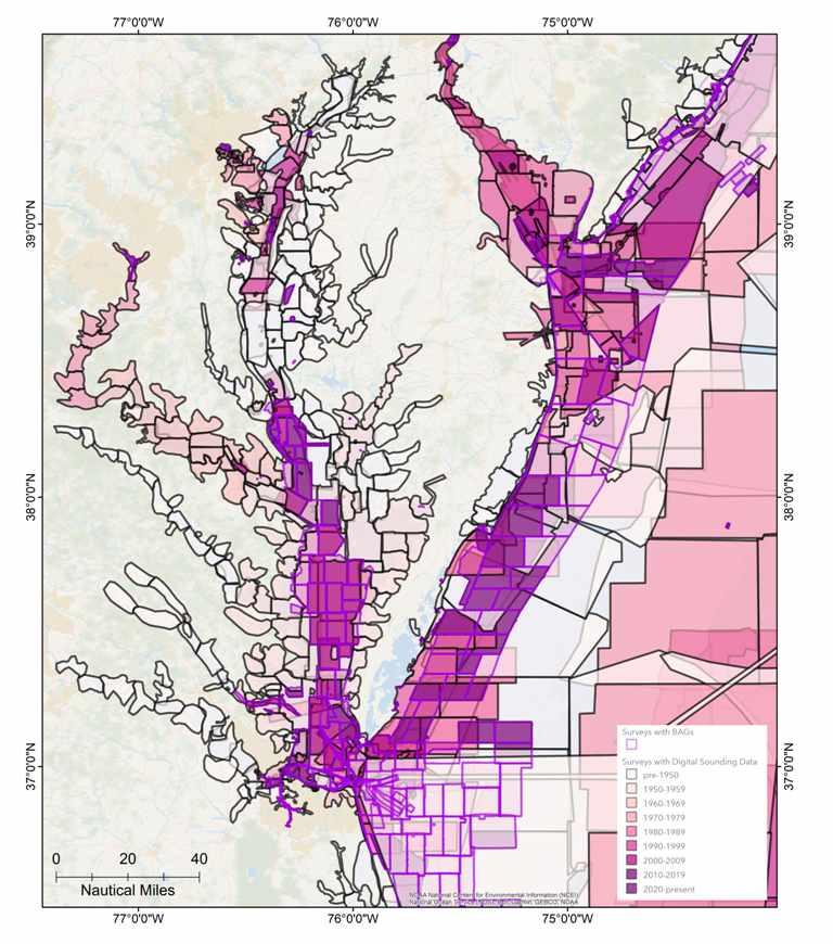
The proposed enhancements to the HHM are implemented and evaluated as a proof of concept study in Chesapeake Bay and nearby Delmarva Peninsula where frequent hydrographic surveys are required to monitor significant sediment transport in heavily trafficked regions (Figure 1). This work creates a link between hydrodynamic models and hydrographic survey priorities that more objectively prioritizes current and future survey needs and investments.
2. Methods
2.1 Initial Survey Uncertainty Calculation
Publicly available data from MarineCadastre.gov and NOAA National Centers for Environmental Information (NCEI – formerly NGCDC; NGDC, 1999) were used in ESRI ArcGIS 10.5.1 and MATLAB 2017b 9.3.0 to perform the σinitial calculation.
All bathymetric data in the study area were downloaded and broken up into layers based on coverage through time and then again into groups based on physical location to lessen processing load and ensure areas of similar natural geophysical processes were processed similarly. Specifically, data were broken into three layers according to initial coverage of the study area and acquisition year (lower, middle, and upper) where the lowest layer includes any dataset that covers a portion of the study for the first time, the upper layer includes the most modern datasets, and the middle includes any data in between. Both the lower and middle layers were further divided into groups based on location for quicker processing (e.g., Upper Chesapeake Bay, Delaware Bay, Delmarva Peninsula, Chesapeake Bay mouth, middle Chesapeake Bay, etc.).
Each group of points was then run through ArcGIS’s kriging tools (discussed in Oliver and Webster, 2014) to interpolate a 40m surface using variogram analyses. Kriging is a well-established, well understood technique for geospatial interpolation (Cressie, 1990; Oliver and Webster, 2014), which has the significant benefit of providing an assessment of the uncertainty of the interpolated surface based on the observed variability of the source data (Calder, 2006; Dorst, 2009; Baily et al., 2010, Aykut et al., 2013). While many other interpolation techniques are possible, providing a usable uncertainty which includes both measurement uncertainty and spatial variability estimates is a significant benefit in the current work. Kriging assumes a number of features of the data, such as ergodicity (one sample of data acts as a proxy for the population) and homogeneity (statistics are stationary from place to place). Very few real datasets completely meet these requirements, but restrictions to relatively small areas typically get closer to the ideal. We have assumed these conditions apply in the current dataset in order to proceed with the analysis. The bathymetric kriging outputs are then mosaicked back together into individual layer grids using user-defined supersession criteria to maintain the temporal progression of the survey area. The kriging uncertainty of each layer was also determined by taking the square root of each layer’s variance output raster, also 40m.
Using the ArcGIS ‘point to raster’ tool, each layer’s point data were gridded to 30 m raster to preserve the point nature of the datasets and then mosaicked with a constant value raster (-999). Th en, the ArcGIS ‘Extract by Attributes’ tool was used to identify the interpolated data. The interpolated data outline was then used as the mask in the ‘Extract by Mask’ tool with the merged layer bathymetry as the base to produce a bathymetric grid of only interpolated data.
All publicly available AIS tracklines were brought into ArcGIS and turned into shapefiles and clipped to the study area. The attribute tables for these shapefiles were exported to Excel tables and brought into a MATLAB workspace. A MATLAB script was created and run to correct errors with draft recordings by identifying excessively large draft values based on vessel type. The underlying assumption being that these values have unit errors and were mistakenly recorded in US feet instead of the required SI meters and thus require conversion. Drafts equal to less than the maximum allowable for each vessel type were not altered. All edited drafts were combined into a singular file, imported back into ArcGIS, and were used to populate a raster grid with the deepest recorded drafts per cell (Figure 2A).
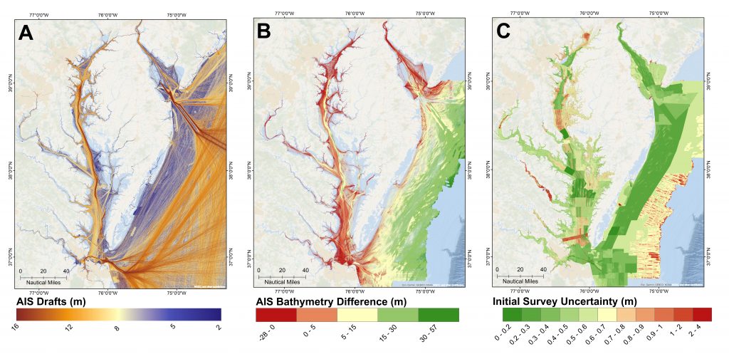
Next, the interpolated bathymetry raster grid for each layer was differenced with the combined draft grid using the ‘Raster Calculator’ tool to determine the vertical distance between the vessel drafts and the seafloor. Any negative values (or positive if depth is negative) are removed as the drafts exceed the bathymetry (discussed further in later sections). The resulting AIS seafloor difference rasters for each layer were differenced from their respective uncertainty raster in the ‘Raster Calculator’ tool to produce a constrained estimate of uncertainty (Figure 2B). Finally, each layer’s constrained uncertainty raster was mosaicked with their original uncertainty raster for a final layer uncertainty grid – constrained uncertainty having priority in the gridding process. These layer uncertainty grids were then mosaicked into one raster with the oldest data on the bottom and the newest data with the highest priority to mimic chart compilation techniques, producing a final estimate of initial survey uncertainties (Figure 2C).
2.2 The HUG Calculation
Publicly available data from NOAA’s Office of Coast Survey’s chart catalog, NCEI bathymetry, and Coastal Relief Model (CRM; NGDC, 1999) bathymetry websites were used in ESRI ArcGIS 10.5.1 and ESRI S-57 Viewer 2.2.0.9 to perform the HUG calculation.
All survey polygons from Electronic Navigation Charts (ENCs) within the study area were used to create constant value survey raster grids populated with survey year. Where surveys existed without polygons, the ‘Raster Domain’ tool was used to create a polygon which was then populated with the survey year and converted to a raster grid. All survey year grids were mosaicked into a combined raster grid of survey age – youngest on top, oldest on the bottom (output similar to Figure 1).
For this study, our temporal variability components were based on sedimentation rates determined by a literature review and bathymetric differencing. All literature review sedimentation rates were translated into a raster grid (with units of m/yr). Bathymetric differencing was performed where overlapping surveys existed by differencing older surveys from more recent surveys and dividing the residuals by the difference in survey year to determine sedimentation rates (in m/yr). Both sets of sedimentation rates were mosaicked into a singular grid (in m/yr) (Figure 3A).
Using the sedimentation rate raster, the survey age raster, and the final constrained initial uncertainty raster, σpresent was calculated in the ‘Raster Calculator’ tool as outlined in (5) (Figure 3C).
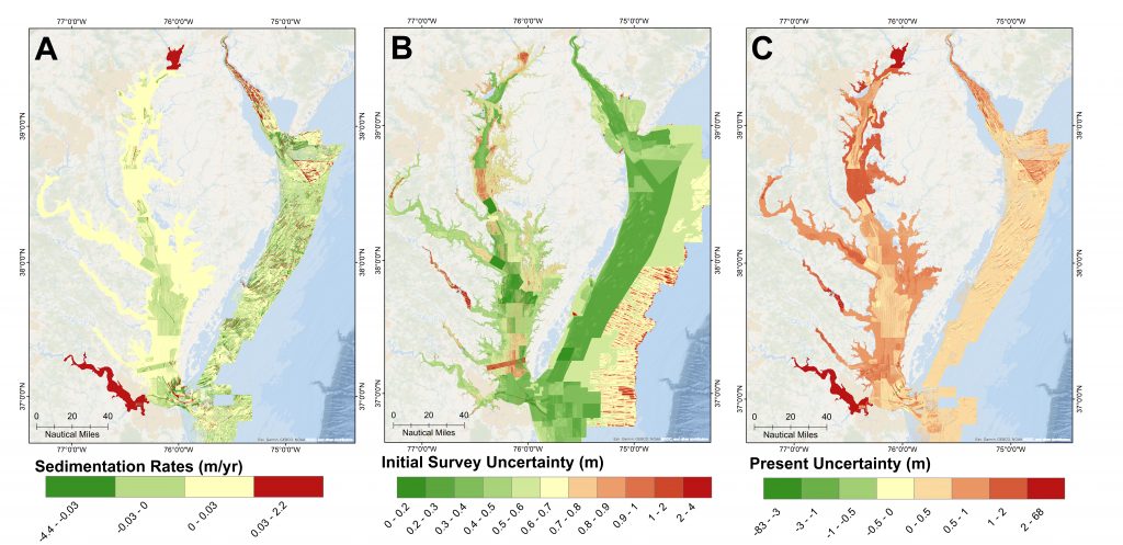
B) HUG Initial survey uncertainty in meters (same as Figure 2C).
C) HUG present survey uncertainty calculated using Equation 4 (Table 1)
and layers shown in A and B. All outputs have 40 m resolution. All figures were made in ArcGIS 10.5.
The HUG equation (4) was performed using the appropriate grids using the ‘Raster Calculator’ tool (Figure 4C). Larger positive values indicate higher survey priorities.
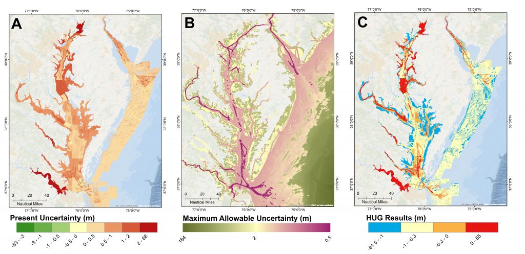
B) HUG maximum allowable uncertainty in meters as defined by NOAA’s HHM. C) HUG final results in meters created using Equation 4 (Table 1)
and the layers shown in A and B. All outputs have 40 m resolution. All figures were made in ArcGIS 10.5.
3. Results
3.1 Initial Uncertainty
Only two years of AIS data were publicly available (2011 and 2013) at the time of this study. Of these, 22% from each year were removed before processing as draft information was not included. Another 10% of the total data were altered through the draft assessment process (i.e. adjusting drafts based on maximum allowable drafts by boat type)– 7% from 2011 and 13% from 2013, primarily from tugboats (Figure 2A). An additional filtering process was performed in ArcGIS during the AIS and bathymetry differencing where 8% of drafts exceeded the bathymetry
(Figure 2B). These data were almost exclusively removed from nearshore areas and within navigational channels both of which could be explained by physical changes to the seafloor between the time of survey and AIS data observation (explored further in later sections). A final initial uncertainty grid revealed that 2% of the total study area was constrained through this process, equating to ~182 nm2 (Figure 2C). Most of the constrained uncertainty values were less than 0.5 m; however, those greater than 0.5 m were observed primarily in areas where the water depth far exceeded two times the uncertainty, and thus were localized to deeper areas where navigational significance is of lesser importance. A small percentage of these are the exception and were found to be exclusively in two surveys (H10193 and D00052) with minimal coverage.
3.2 Present Uncertainty
Sedimentation rates were estimated for the entire study area from reported values and bathy-metric differencing for areas with repeat surveys. The combined average rate was +2.8 mm/yr and only 16% of the study had rates over 10 mm/yr, the majority of which are found offshore and in Delaware Bay (Figure 3A). The largest reported rates were observed at the Susquehanna and James Rivers within Chesapeake Bay while the largest bathymetric differencing rates were found at the mouth of Chesapeake Bay. The latter is consistent with the findings presented by Colman et al. (1988) where shoal sediments are worked into the bay by Fisherman’s Island and into the channels in a south-western progression. Similar patterns are observed at the mouth of Delaware Bay around Cape May. Similarly, offshore Delmarva exhibits sedimentation rate patterns consistent with migration along the coast evident by the presence of positive values (areas of deposition) contiguous with negative values (areas of erosion) with rates that fall near
± 20 mm/yr.
Both final sedimentation rate (Figure 3A) and initial uncertainty (Figure 3B) raster grids are used to fully estimate the present state of hydrographic data within the study area. The average present uncertainty was 0.66 m with a standard deviation of 0.87 m (Figure 3C). Over 47% of the study area has uncertainty larger than 0.5 m, but only 15% has uncertainty larger than 1 m and 18% larger than 50% of the water depth. The largest uncertainties are found in and around the Susquehanna and James Rivers as a direct result of large sedimentation rates and survey ages. The values produced in these areas by this model are not realistic and instead are a byproduct of inaccurately capturing the true nature of geophysical processes, not accounting for dredging, and sparse bathymetric coverages. However, they still call attention to a region of large change and high uncertainty in the current information.
3.3 Hydrographic Uncertainty Gap
The user-defined σmax was determined for this study by translating the current HHM DSS values into uncertainty values aligned with CATZOC TVU calculations allowing a direct comparison of final HUG results between the two models (Figure 4B). This maximum uncertainty raster was then subtracted from the final present uncertainty (Figure 4A) to create the HUG outputs (Figure 4C). The average result was a gap of -0.40 m with a standard deviation of 0.91 m. The lowest observed values were found in intertidal zones in central Chesapeake Bay. The maximum values were near navigational channels in both bays, upstream of the major rivers in Chesapeake Bay, and around the mouth of Chesapeake Bay. Only 13.6% of the study area exceeds the maximum uncertainty and were determined survey priorities – equal to nearly 1,130 nm2. About 80% of these priorities have uncertainties that are less than 50% of the water depth, although 215 nm2 exceed this and are found near the Susquehanna and James Rivers.
4. Discussion
4.1 HUG Ambiguity
While our methodology provides a prioritized assessment of the study area regarding survey investments, possible sources of ambiguity may be found in two key assumptions essential to HUG model development.
Negative values were calculated through the differencing of AIS drafts and bathymetry. These negative values were filtered out as ambiguous data and through elimination provides a more conservative estimate. In this process we could not account for tides, smaller unit errors or misassignment of vessel category embedded in the AIS information, nor changes in bathymetry through time. Given the nearly 290,000 AIS tracklines available across both 2011 and 2013 datasets, it would be an arduous task to verify each attribution for every vessel without error. Similarly, determining which vessels advantageously used the tides to gain access would be hard to incorporate accurately in this workflow without adjusting every ship passage to account for tides.
That said, the tides within the study area have an observed maximum of ~1 m above MLLW and the difference between MLLW and MSL is less than 0.5 m. While this is still enough to change the model outputs, leaving the AIS drafts referenced to MSL provides a more conservative uncertainty than if everything was referenced to MLLW. Specifically, referencing to MLLW would increase the number of apparent groundings, ultimately removing more data from the analysis due to ambiguity; what does not ground makes the uncertainty smaller. Conversely, if drafts are referenced to MHHW, the uncertainties become more conservative, but allow for larger errors in AIS drafts to be perpetuated by increasing the draft limits. Thus, referencing drafts to MSL minimizes errors in both the AIS drafts and the uncertainties.
Perhaps the most impactful aspect of this assumption comes from our inability to account for temporal variability. The only public AIS information is from 2011 and 2013, but the bulk of the data incorporated into this calculation comes from the 1940-1960s. It is highly probable that the seafloor has changed within the last 50 years, especially given the creation and constant maintenance of deep-draft navigational channels throughout the study area since the 1800s (Gottschalk, 1945; Hargis, 1962). While it is also possible that these locations represent navigational hazards, if groundings had occurred, the charts in these areas would have changed to reflect this and additional more modern bathymetry would have been gathered. As such, it is most likely these data represent errors from draft recordings or changes in bathymetry not reflected in historic data, so they were removed.
Along similar lines, we presume to accurately account for temporal variability through sedimentation rates and bathymetric differencing. While bathymetric differencing is not new and has been done many times before (Ludwick 1978; Donoghue, 1990; Hobbs et al., 1990; Van Der Wal and Pye, 2003), assumptions are required including that all data used are without error, yet depth and position errors can propagate through the analysis and lead to misinterpretations (Van Der Wal and Pye, 2003; Jakobsson et al., 2005). Additionally, bathymetric differencing can lead to inaccurate predictions including those derived from migratory rates which may only be valid for a specific point in time, as sand waves, dunes, shoals, and bars oscillate shoreward and offshore depending on wave energy (e.g., Gallagher et al., 1998; and many others).
HUG estimates resulting from this approach may not quantify all geophysical processes acting on the study area, especially in regards to dredging activities; however, they are inclusive of high-frequency changes like effects from tides, storms, and flooding and do still identify areas of potential change (Van Der Wal and Pye, 2003). Future work should focus on the inclusion of known migratory rates and patterns into sedimentation rate calculations. Additionally, temporal variability estimates could further be improved with outputs from sediment transport models.
The methodology discussed in this paper allows for reliable sediment transport model predictions to be directly input into the HUG model via the temporal variable in (5) and can ultimately be used to identify future survey priorities with more certainty in areas with large changes and complex forcing.
4.2 Direct comparison with HHM Hgap results
In order to assess the HUG outputs, a direct comparison with the HHM Hgap outputs in our study area was performed. In this study, we translated the HHM ISS and DSS values using the IHO CATZOC levels as indicated by the coverage requirements for each ISS and DSS level (Table 1). Using CATZOC levels and TVU variables outlined in Table 1, an HHM Initial Survey Score (ISS) uncertainty grid was created and compared to the HUG final initial survey uncertainty grid (Figure 5). 88% of the σinitial uncertainties are smaller than those from the ISS. The largest uncertainties resulted from an edging effect due to resolution differences between the two models and from a few more modern surveys. As coarser grids populate larger geospatial areas with single values, finer grids allow for more variability to be captured and comparing the two can result in large differences particularly on the outer edges of each grid.
It is not wholly surprising that the HHM ISS uncertainty values would be larger, as charts are compiled from conservative estimates of uncertainty and shoal-biased bathymetric grids (Van Der Wal and Pye, 2003; Wong et al., 2007; NOAA, 2018) compounding “worse case” scenarios for increased safety margins. In particular, the assignment of a CATZOC level is itself a conservative process where the limiting factor between coverage and data quality determines the confidence level for the whole survey area (Calder, 2006; IHO S-57, 2014). This process unintentionally implies that the seafloor contained within the bounds of each survey polygon meets the corresponding level uncertainties which is not always the case. As the uncertainty of hydrographic data is only known where data exists and cannot accurately be extrapolated between data points, it is not uncommon for data to have larger uncertainties than can be estimated without accounting for geophysical processes (Calder, 2006; Oliver and Webster, 2014). Thus, the methodologies outlined in this paper provide more accurate initial uncertainty estimates as a direct result from utilizing the uncertainties associated with each survey and calculating the uncertainty between bathymetric data points instead of generalizing an area by its lowest quality.
As previously mentioned, the PSS decay coefficient in (3) uses heuristic estimates to highlight areas of potential physical change; however, this calculation produces values that cannot be translated to uncertainty and therefore a direct comparison between the PSS and σpresent terms is not possible. Given that the DSS and σmax values are essentially the same, a direct comparison of Hgap and HUG outputs almost exclusively addresses this comparison. With that in mind, 52% of Hgap values are greater than 0 and indicate hydrographic “needs” (Keown et al., 2016; Fandel et al., 2017; Hicks et al. 2017). This is almost four times more than the 13.6% identified by the HUG model and is potentially a result of over-estimating risk and underestimating survey quality but is also a direct result of the differences in the PSS calculation.
Specifically, the HHM attributions of “CATZOC” for both the ISS and DSS variables do not equate to the traditional international CATZOC TVU standards alone, but also incorporate the seafloor coverage and survey characteristics portions of the CATZOC definition as well. From the TVU-derived definition alone, this leads to a conservative grouping of the CATZOC values (Table 2). For example: a survey that meets or exceeds CATZOC A1 standards initially is then grouped with surveys that meet CATZOC A2 standards. This is inherently a conservative process as CATZOC A1 and A2 have vertical and horizontal uncertainty requirements double of each other and very different coverage requirements, meaning any survey that meets A1 would be indistinguishable from A2 surveys in the HHM outputs despite meeting stricter requirements. These A1/A2 surveys would then undergo conservative estimates of physical change and then potentially be compared to NOAA’s object detection standards. HHM accounts for this by differentiating the ISS for surveys depending on their degree of bottom coverage.
Arguably, more accurate HHM results could be achieved by grouping surveys strictly on their uncertainty requirements, which would leave A1 surveys in a group of their own and then group A2 and B surveys together as their uncertainty requirements are the same, an issue that was highlighted through the translation process of the HHM groups into the HUG model. If the HHM process remains unchanged, it will always produce large amounts of survey priorities based on the assignment of initial survey quality.
Table 2

Table 2: HHM ISS and DSS groups and their assigned CATZOC level and correspondin TVU values in comparison with the traditional CATZOC and TVU values. *CATZOC <A1 does not exist internationally, it is a NOAA standard found in their Hydrographic Survey Specifications and Deliverables Document (NOAA, 2018) and the corresponding TVU variables are estimated by the authors. All other TVU are from the International Hydrographic Organization (IHO) S-44 quality standards for assessing survey uncertainty later applied through S-57 Category of Zones of Confidence (CATZOC) Levels.
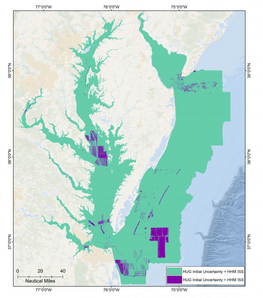
Figure 5: HHM ISS comparison with HUG initial uncertainty estimates. Teal represents where HUG values are less than HHM ISS estimates, and purple indicates where HUG values are greater. Figure created in ESRI ArcGIS 10.5
There is an argument to be made that identifying 52% of the study area as survey needs does not identify priorities but instead highlights a lack of information necessary to make priority-based decisions. However, when focusing on Hgap values that exceed a health rating of 50, only 14% of the area were identified which is a more comparable quantity to the identified HUG priorities but lacks the consistent overlap (Figure 6). Only 30% of the Hgap values over 50 overlap with HUG priorities, leaving almost 300 nm2 of unique HUG survey priorities.
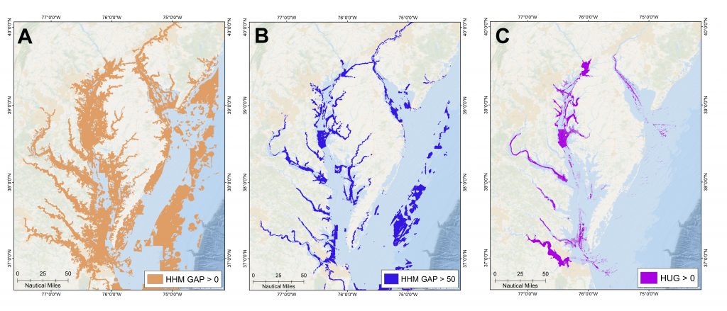
Figure 6: A) NOAA HHM Hgap values in the study area greater than zero, which show survey needs. B) NOAA HHM Hgap values greater than 50 (as an example chosen to denote possible survey priorities). C) HUG values greater than zero which equate to survey priorities. HHM outputs have 500 m resolutions and the HUG outputs have 40 m resolution.
All figures were made in ESRI ArcGIS 10.5.
When looking at the notoriously problematic navigation channels throughout the study area (Gottschalk, 1945; U.S. Army Corps of Engineers, 2017), almost all are identified in the HUG priorities and none are visible in the HHM. This is likely a result of resolution differences – the HHM has an output resolution of 500 m and the HUG output is 40 m. While the 500 m HHM resolution makes modeling on a national scale more achievable, it misses the small-scale features essential to safe navigation. Additionally, the HUG priorities encapsulate known problem areas like the eastern side of the mouth of Chesapeake Bay, an area fed by shelf sediments that extend into the bay along the eastern boundary and are driven by a strong longshore current from the Delmarva Peninsula (Coleman et al., 1988). This is supported by U.S.G.S. mobility estimates that show greater sediment movement on the eastern side of the bay than those observed on the western side (Dalyander et al., 2013).
Conversely, the HHM priorities are primarily grouped on the western side of the bay, north of and including the James River mouth. While the James River is known for large sedimentation rates and has been found to be the primary source of infilling in the southern Chesapeake Bay mouth channels (Ludwick, 1981; Donoghue, 1990; Skrabal et al., 1991), this does not explain the continued western favoritism the HHM priorities exhibit. Instead, the answer is again found in how each model accounts for change. The HHM decay coefficient’s use of heuristic change estimates is likely to have overestimated how influential storms and tidal currents are on the western half of the bay while underestimating original data quality. While limited available geologic information supports the results from the HHM, the only way to truly verify either model’s results would be to survey a portion of their priority areas to ground truth and calibrate future iterations.
4.3 Recommendations for national-scale implementation
The HHM is NOAA’s national model for estimating survey priorities and a large part of its feasibi-lity is that its output resolution is lowered to 500 m. Such low resolution does not capture complex geophysical processes and features essential to safe navigation. Conversely, the HUG model presented in this paper has an output resolution of 40 m which allows for these more detailed analyses, although would be problematic to maintain when scaling nationally. That said, not all regions within the coastal U.S. are faced with the same dynamic processes as those highlighted in our study area and consequently do not require analyses to the same level of detail. Thus, we recommend a variable resolution output for national implementation where complex areas (such as navigable inlets and shoals) have higher resolution outputs and more steady areas (such as offshore in deeper waters) have lower resolution outputs.
Problem areas within the U.S. are well known to NOAA hydrographers, who typically consult with local stakeholders in determining final survey areas and schedules, so determining where higher-resolution outputs should be incorporated into the model itself should be a fairly straightforward process. For example, Louisiana consistently struggles with the Mississippi River delta (Mossa, 1996; Nittrouer et al., 2008; Nittrouer et al., 2012) and the outputs from the Columbia River on the border of Washington and Oregon are also problematic with sediment moving along the coast (Byrnes and Li, 1996; Kaminsky et al., 2010). These places and others are long-established problem areas that have drawn the attention of local scientists, meaning extensive archives of geophysical studies may be readily available. Furthermore, locations of heightened interest may have already established coupled hydrodynamic and sediment transport models in place, the outputs of which could be directly incorporated into the HUG calculations.
While it is more time-consuming to collaborate with outside groups, incorporate third-party outputs, and perform extensive studies on all known high-risk areas, such efforts would yield model results more aligned with the actual behavior. Once a base understanding for each area is established, future iterations should take less time. Consideration of the extra time required for these advance analyses should be balanced with the time and money necessary to survey – the more accurate the model, the less likely that limited survey resources would be expended on surveying areas unnecessarily. Regardless, the methodology outlined in this paper provides a pathway for the inclusion of more realistic estimates of change and should be considered as part of the Hgap. As such, we recommend incorporating hydrodynamic outputs from established models where appropriate nationally to include in future HUG calculations.
5. Conclusion
An alternative quantitative approach for identifying survey priorities is presented. Specifically, we outline methods to calculate and constrain vertical uncertainty of less-than full coverage hydrographic surveys using AIS records and kriging, and how to incorporate quantifiable hydrodynamic estimates of change through an updated hydrographic gap calculation. A proof-of-concept study was implemented in and around Chesapeake Bay, Delaware Bay, and the Delmarva peninsula, and compared with NOAA’s current HHM outputs. Through this example we demonstrate the potential improvement by including more complex and quantifiable estimates of change with
applications at national scale. We also recommend variable resolution outputs for regional scale models and how inclusion of existing verified hydrodynamic and sediment transport models can be used for bathymetric change predictions.
6. Acknowledgements
The scientific results and conclusions, as well as any views of opinions expressed herein, are those of the author(s) and do not necessarily reflect the views of NOAA or the Department of Commerce.
This work was fully funded by NOAA grant NA15NOS4000200. The authors would like to thank Christy Fandel, Patrick Keown, and Corey Allen of NOAA Office of Coast Survey for their input and assistance on this project.
7. References
– Adams, K.T. (1942). Hydrographic Manual. U.S. Department of Commerce, Coast and
Geodetic Survey. Special Publication No. 143.
– Aykut, N. O., Akpinar, B., Aydin, O., (2013). “Hydrographic data modeling methods for determining precise seafloor topography”, Computational Geosciences, 17(4), pp. 661-669.
– Bailey, J., Le Coarer, Y., Languille, P., Stigermark, C., and Allouis, T., 2010, “Geostatistical estimations of bathymetric LiDAr errors on rivers”, Earth Surface Processes and Landforms, 35, pp. 1199-1210.
– Calder, B. (2006). “On the Uncertainty of Archive Hydrographic Data Sets”, IEEE Journal of Oceanic Engineering, 31(2), pp. 249-265.
– Colman, S., Berquist Jr., C.R., and Hobbs, C.H. (1988). “Structure, Age and Origin of the
Bay-Mouth Shoal Deposits, Chesapeake Bay, Virginia”, Marine Geology, 83, pp. 95-113.
– Cressie, N. (1990). “The origins of Kriging”, Mathematical Geology, 22(3), pp. 239-252.
– Dalyander, P.S., Butman, B., Sherwood, C.R., Signell, R.P., and Wilkin, J. (2013). “Characterizing wave- and current- induced bottom shear stress: U.S. middle Atlantic continental shelf”, Continental Shelf Research, 52, pp. 73-86.
– Donoghue, J.F. (1990). “Trends in Chesapeake Bay Sedimentation Rates during the Late
Holocene”, Quaternary Research, 34, pp. 33-46.
– Dorst, L. L., Roos, P. C., Hulscher, S., Lindenbergh, R. C., (2009). “The estimation of sea floor dynamics from bathymetric surveys of a sand wave area”, Journal of Applied Geodesy, 3(2), pp. 97-120.
– Fandel, C., Allen, C., Gallagher, B., Gonsalves, M., Hick, L., and Keown, P. (2017). “Desire, decay, and risk: Establishing survey priorities through the assessment of hydrographic health”, NOAA Field Procedures Workshop, Virginia Beach, VA, USA, NOAA.
– Gallagher, E.L., Elgar, S., and Guza, R.T. (1998). “Observations of sand bar evolution on a natural beach”, Journal of Geophysical Research, 103(C2), pp. 3203-3215.
– Gonsalves, M., Brunt, D., Fandel, C., and Keown, P. (2015). “A Risk-based Methodology of Assessing the Adequacy of Charting Products in the Arctic Region: Identifying the Survey Priorities of the Future”, U.S. Hydrographic Conference 2015, National Harbor, MD, USA, pp. 1-20.
– Gottschalk, L. (1945). “Effects of Soil Erosion on Navigation in Upper Chesapeake Bay”, Geographical Review, 35(2), pp. 219-238.
– Hargis, W. J. (1962). “History and Current Status: James River Navigation Project”, Special Reports in Applied Marine Science and Ocean Engineering (SRAMSOE) No. 2, Virginia Institute of Marine Science, College of William and Mary. https://doi.org/10.21220/V5GH99
– Hawley, J.H. (1931). Hydrographic Manual. U.S. Department of Commerce, U.S. Coast and Geodetic Survey. Special Publication No. 143.
– Hicks, L., Gonsalves, M., Allen, C., Fandel, C., Gallagher, B., and Keown, P. (2017). “Incorporating vessel traffic in an assessment of hydrographic health”, Environmental Data Management Workshop, Silver Spring, MD, USA.
– Hobbs, C. H., Halka, J. P., Kerhin, R. T., and Carron, M. J. (1990). “A 100-Year Sediment Budget for Chesapeake Bay”, Special Reports in Applied Marine Science and Ocean Engineering (SRAMSOE) No. 307. Virginia Institute of Marine Science, William & Mary. https://doi.org/10.21220/V5RX6S
– IHO S-44 (2008). IHO Standards for Hydrographic Surveys, Special Publication 44, 5th Edition, Monaco.
– IHO S-57 (2014). The IHO Transfer Standard for Digital Hydrographic Data: Supplementary Information for the Encoding of S-57 Edition 3.1, ENC Data June 2014. International Hydrographic Bureau Monaco S-57 Supplement No. 3, pp. 1-4.
– Jakobsson, M., Armstrong, A., Calder, B., Huff, L., Mayer, L., and Ward, L. (2005). “On the Use of Historical Bathymetric Data to Determine Changes in Bathymetry: An Analysis of
Errors and Application to Great Bay Estuary, NH”, International Hydrographic Review, 6 (3), pp. 25-41.
– Keown, P., Gonsalves, M., Allen, C., Fandel, C., Gallagher, B., and Hicks, L. (2016). “A risk-based approach to determine hydrographic survey priorities using GIS”, 2016 ESRI Ocean GIS Forum, Redlands, California, USA.
– Ludwick, J.C. (1978). “Coastal Currents and an Associated Sand Stream off Virginia Beach, Virginia”, Journal of Geophysical Research, 83(C5), pp. 2365-2372.
– Ludwick, J.C. (1981). “Bottom sediments and depositional rates near Thimble Shoal Channel, lower Chesapeake Bay, Virginia”, GSA Bulletin, 92 (1), pp. 496-506.
– Mossa, J. (1996). “Sediment dynamics in the lowermost Mississippi River”, Engineering Geology, 45, pp. 457-479.
– NGDC (1999). U.S. Coastal Relief Model – Southeast Atlantic. National Geophysical Data Center, NOAA. doi:10.7289/V53R0QR5.
– Nittrouer, J.A., Allison, M.A., and Campanella, R. (2008). “Bedform transport rates for the lowermost Mississippi River”, Journal of Geophysical Research, 113, no. F03004, pp. 1-16.
– Nittrouer, J.A., Shaw, J., Lamb, M., and Mohrig, D. (2012). “Spatial and temporal trends for water-flow velocity and bed-material sediment transport in the lower Mississippi River”, GSA Bulletin, 124(3/4), pp. 400-414.
– NOAA (2018). Hydrographic Survey Specifications and Deliverables, National Oceanographic and Atmospheric Administration, Office of Coast Survey, viewed 30 August 2017, https://nauticalcharts.noaa.gov/publications/standards-and-requirements.html.
– Oliver, M.A., and Webster, R. (2014). “A tutorial guide to geostatistics: Computing and modelling variograms and kriging”, Catena, 113, pp. 56-69.
– Skrabal, S. (1991). “Clay mineral distributions and source discrimination of upper Quaternary sediments, lower Chesapeake Bay, Virginia”, Estuaries, 14 (1), pp. 29-37.
– Taylor, J.R. (1982). An Introduction to Error Analysis: The Study of Uncertainties in Physical Measurements, Second Edition, University Science Books, Mill Valley, California.
– U.S. Army Corps of Engineers (2017). Norfolk Harbor Navigation Improvements: DRAFT General Reevaluation Report and Environmental Assessment. U.S. Army Corps of Engineers, USA.
– Van Der Wal, D., and Pye, K. (2003). “The use of historical bathymetric charts in a GIS to assess morphological change in estuaries”, The Geographical Journal, 169(1), pp. 21-31.
– Wong, A.M., Campagnoli, J.G., and Cole, M.A. (2007). “Assessing 155 Years of Hydrographic Survey Data for High Resolution Bathymetry Grids”, IEEE OCEANS 2007, Vancouver, BC, Canada, pp. 1-8.
8. Author Biographies
Cassandra Bongiovanni has B.S. in Geology from the University of Washington and a M.S. in Ocean Mapping from the Center for Coastal and Ocean Mapping at the University of New Hampshire. She has worked for NOAA on post-Hurricane Sandy hydrographic data analysis for charting, and as the director of mapping operations for private deep-sea exploration expeditions. Her research interests include marine geology, uncertainty of bathymetric data through time, and global tectonics.
Email: cassie.bongiovanni@gmail.com
Dr. Tom Lippmann is an Associate Professor in the Dept. of Earth Sciences at the University of New Hampshire. He received his PhD in Oceanography from Oregon State University in 1992. He is also affiliated with the Center for Coastal and Ocean Mapping, a Joint Hydrographic Center with NOAA. He is the Director of the Oceanography Graduate Program, and a member of the School of Marine Science and Ocean Engineering. His research is focused on field observations, bathymetric mapping, and numerical modeling of shallow water marine processes associa-ted with inlets, estuaries, beaches, and coastlines.
Email: t.lippmann@unh.edu
Dr. Brian Calder is a Research Assistant Professor at the Center for Coastal and Ocean Mapping & Joint Hydrographic Center at the University of New Hampshire. He graduated MEng and PhD in Electrical & Electronic Engineering from Heriot-Watt University in Edinburgh, Scotland in 1994 and 1997 respectively, but was subsequently seduced into sonar signal processing for reasons that are now obscure. His research interests have previously covered speech recognition, texture analysis, object detection in sidescan sonar, high-resolution sub-bottom profiling, simulation of forward-looking passive infrared images, acoustic modelling and pebble counting. Currently, they revolve around the application of statistical models to the problem of hydrographic data processing.
Email: brc@ccom.unh.edu
Captain Andrew Armstrong, NOAA (retired) is the NOAA Co-Director of the Joint Hydrogra-phic Center at the University of New Hampshire. Along with the UNH Co-Director, he manages the research and educational programs of the Center. He is a past President of the Hydrographic Society of America and past Chair of the FIG/IHO/ICA International Board on Standards of
Competence. Captain Armstrong has over 30 years of hydrographic experience with NOAA, including positions as Officer in Charge of hydrographic field parties, Commanding Officer of NOAA Ship Whiting, and Chief, Hydrographic Surveys Division.
Email: andy.armstrong@noaa.gov