

Abstract
1. INTRODUCTION
The Federal Maritime and Hydrographic Agency (BSH) of Germany collects bathymetry and detects underwater obstructions from vessel-mounted multibeam systems (Dehling and Ellmer 2012). For the purpose of safety of surface navigation at sea, bathymetry data collected by multibeam echosounders in German offshore waters is expected to meet IHO S-44 Order 1a survey requirements (IHO 2020) before being processed into official nautical charts and publications. While these survey requirements are presently fit for purpose, the combination of expected higher-density marine traffic in shallow navigable waters and an expanding client base wishing to use bathymetric products for other purposes than safety of navigation warrants the adherence to and fulfillment of more stringent survey requirements. This objective is also well in line with geo- detic and hydrographic considerations aiming to minimize all possible single error sources which can be empirically modeled.
An important error source in multibeam systems is the sound speed error which affects the beam range and angle (i.e. beam vector) determination in two distinct ways (Dinn, Loncarevic, and Costello 1995; Tonchia and Bisquay 1996): 1) the sound speed at the multibeam antenna arrays determines the along-track (for the transmitter) and across-track (for the receiver) directivity pattern steering angles, the intersection of which corresponds to the array relative beam pointing angle; 2) the sound speed scalar field in the water column determines, together with the measured two-way travel time and the initial beam launch angle, the refracted path followed by the acoustic ray between the multibeam and the seafloor. Any sound speed measurement error will therefore affect the beam vector determination and propagate to the final 3D point solution referenced in a terrestrial reference frame. Beam vectors with high launch angles (low depression angles) are especially sensitive to these error sources.
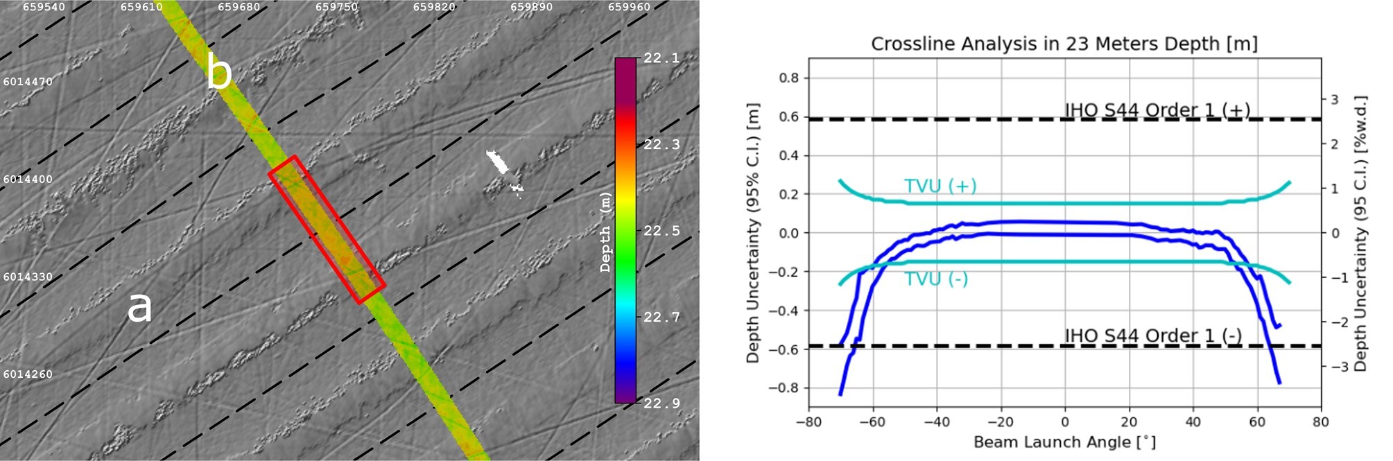
Recent multibeam surveys conducted by BSH in the southern Baltic Sea have been documented as being affected by an angular dependent error classifiable as a type IV error (Hughes Clarke 2003). Figure 1 illustrates the impact of this error which is hypothesized as being sound speed induced. Although the IHO Order 1a depth uncertainty requirement is fully achieved within the ±65° interval in this illustrative example, the depth uncertainty above and below the ±50° interval exceeds the depth uncertainty budget of the multibeam system (cyan curves in Figure 1). This in turn limits the usable multibeam swath, which translates to the need for even tighter line spacing in order to achieve higher accuracy. In shallow waters, where line spacing is already tight, such demand is often counterproductive.
Approaches to minimize sound speed errors in multibeam data are numerous. Capell (1999) showed that the 45° beam angles are not affected by ray-tracing errors and can thus potentially be used to estimate the measured sound speed profile (SSP) error. Kammerer and Hughes Clarke (2000) developed a post-processing method which uses overlapping parallel or cross- tracks to estimate the ray-tracing coefficients of a simple two-layer water column. Yang et al. (2007) and Ding, Zhou, and Tang (2008) attempt to estimate by inversion a simplified equivalent profile based on overlapping tracks. This method requires knowledge of a best depth estimate which is by default attributed to the nadir beams. However nadir beams are also affected by range errors due to harmonic sound speed errors (Dinn, Loncarevic, and Costello 1995; Eeg 1999). Eeg (2010) proposed an optimal estimator on overlapping cross-tracks which seeks to estimate the mean sound speed profile error. More recently, Mohammadloo et al. (2019) proposed two optimization methods based on overlapping parallel tracks that determine by inversion a constant sound speed profile. Although all approaches reviewed here are usable in practice, the additional post-processing overhead required is contrary to the demands of a hydrographic organization is terms of efficiency and up-to-dateness.
While a surface sound speed sensor necessary for beam steering may have a typical sampling period of 50 ms and a reported accuracy of 0.05 m/s, the sound speed profile sampling period of a typical surveying day of a BSH ship may be in excess of 60 minutes. The only practical way to decrease the sampling period without compromising survey time is to use an underway profiling system. The cost benefit of such systems in terms of survey time and measurement accuracy is well documented (Hughes Clarke, Lamplugh, and Kammerer 2000; Peyton, Beaudoin, and Lamplugh 2009). The challenge with underway profiling systems is rather finding the appropriate sampling period. Indeed the sampling period should ideally be set so as to fully capture the spatiotemporal scale of the oceanographic processes while minimizing the number of measure- ment-cycles. This will minimize excessive wear generated by unnecessary cycles and increase the timespan between recommended maintenances.
If the sound speed profile sampling density is assessed after the survey as being too low, synthe- tic sound speed profiles may be used as substitute to measured profiles. Temperature, salinity and pressure parameters from baroclinic hydrodynamic models can be used to derive such synthetic sound speed profiles applicable to multibeam ray-tracing. The use of such models at global and regional scales has been shown to produce multibeam survey products that comply with IHO survey requirements (Beaudoin, Hughes Clarke, and Bartlett 2006; Calder et al. 2004; Church 2020; Masetti et al. 2020). An alternative approach to derive synthetic sound speed profiles is spatiotemporal prediction1 (i.e. interpolation and sometimes extrapolation) from measured profiles. Indeed, common geospatial interpolation methods (e.g. deterministic, geostatistical) are easily adaptable to higher dimensions (Hengl 2009) and have been applied in oceanographic applications (North and Livingstone 2013; Ridgway, Dunn, and Wilkin 2002). For the purpose of deriving synthetic sound speed profiles, Cartwright and Hughes Clarke (2002) and Church (2020) used linear interpolation. Tollefsen and Pecknold (2010) compared the performance of linear, triangular and trapezoidal interpolation techniques and concluded that the latter two techniques were better suited to track a rising sound speed channel than the linear interpolation technique.
This paper presents an approach for compensating an insufficient sound speed profile sampling density with synthetically-derived sound speed profiles derived from both a regional forecast hydrodynamic model of the Baltic Sea or from spatiotemporal interpolation. Sound speed profiles collected with an underway profiling system are used as a reference dataset for an investigation of the depth accuracy. The approach can be applied independently of the surveyed sound speed profile density and is not based on optimal adjustment of overlapping datasets. As such, achieved performance can be evaluated solely on measured sound speed profiles datasets, as shall be demonstrated. The paper is structured as follows: Section 2 present the survey sensors, collected datasets as well as methods developed; Section 3 presents the depth accuracy assessments when using synthetic sound speed profiles for ray-tracing; Section 4 summarizes the results and presents perspectives for future work; Section 5 presents a brief conclusion.
2. SENSORS, DATA AND TECHNIQUES
A multibeam echosounder was used simultaneously with an underway profiling system to generate the most accurate portrayal possible of the bottom topography (Section 2.1). Normally, an objective accuracy assessment would require comparison to a reference dataset with a higher accuracy order. This requirement is however particularly difficult to achieve in hydrography. As a substitute, the accurate bathymetric model generated using the complete surveyed datasets will serve as reference for statistically meaningful comparisons between real and synthetic profiles. Synthetic sound speed profiles were derived from BSHcmod, a regional hydrodynamic model for the North Sea and Baltic Sea operated by BSH (Section 2.2). Its main present purpose is to pro- vide short-term forecasts for important physical parameters including currents, water levels, temperature, salinity and sea ice coverage. This model has of yet never been used to derive synthetic sound speed profiles in support of hydrographic surveying. Spatiotemporal interpolation is an alternative method to produce synthetic sound speed profiles (Section 2.3). This investigation limits itself to a single parametrizable deterministic four dimensional interpolator. The same comparison procedure based on ray-tracing of sound speed profile pairs is applied regardless of the source of the synthetic profiles (Section 2.4). Making use of both real and synthetic sound speed profiles requires a thoughtful approach and raises several considerations including the appropriate choice of sampling period (Section 2.5).
2.1 Survey Data
Bathymetric data collected from the BSH survey ship VWFS Deneb (Figure 2, left) was used in this investigation. VWFS Deneb is equipped with a Teledyne-RESON Seabat 7125-SV2 400 kHz multibeam which collects the acoustic range and angle data. Attitude and heading solutions are provided by a IXBLUE HYDRINS Inertial Navigation System. Position (inertially-aided) is determined using the same system coupled to a Trimble SPS855 GNSS receiver. GNSS corrections are provided by the national satellite positioning service of Germany, SAPOS (Satellitenpositionierungsdienst der deutschen Landesvermessung). SAPOS’ HEPS solution guarantees a height accuracy of 2-3 cm (SAPOS 2021) allowing real-time kinematic (RTK) surveys (Riecken and Kurtenbach 2017). In June 2020 VWFS Deneb was fitted with an AML Oceanographic MVP-30 underway profiling system (Figure 2, right) equipped with a MVPX SVP&T sensor.
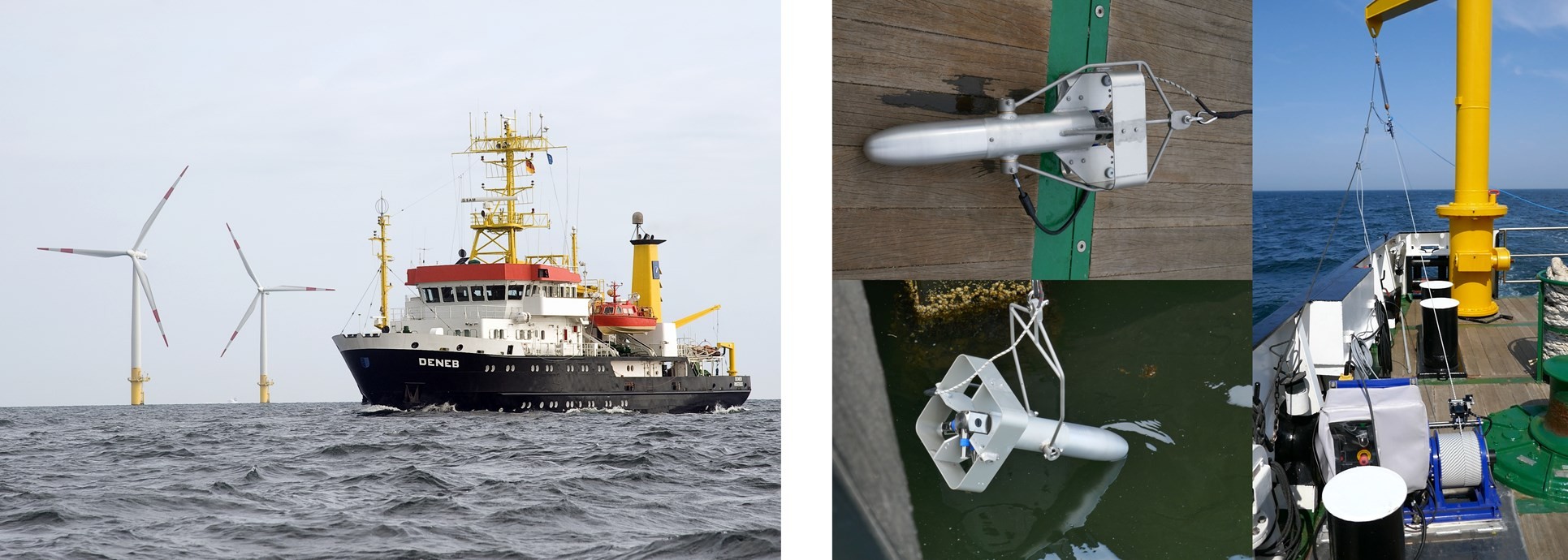
Figure 3 presents the bathymetric models generated from three VWFS Deneb multibeam surveys conducted on July 28th, August 16th and September 14th 2020. All surveys are located in the approach to Rostock (southwestern Baltic Sea). The MVP-30 achieved a mean along-track spatial density of 2.3 sound speed profile per kilometre or, equivalently, a mean period of 2.6 minutes between sound speed profiles. Table 1 presents relevant metadata related to both the bathymetry and the sound speed profiles for each respective survey. All three surveys possess commonalities of location, area, depth, spatial density and temporal density. Variations in the water column stratification are thus assumed to be influenced by local atmospheric and oceanographic conditions.
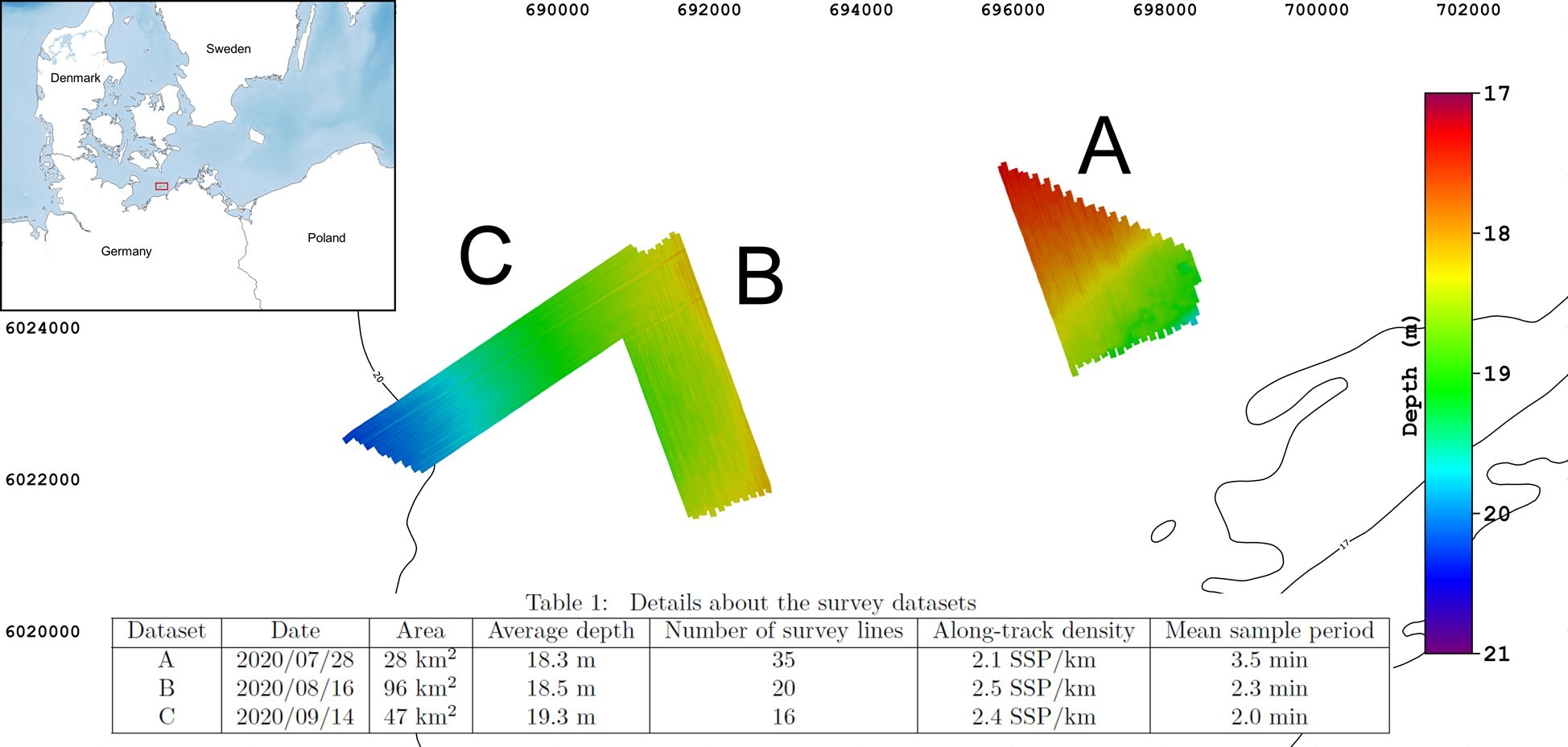
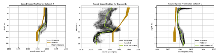
Figure 4 (black curves) clearly shows differences in stratification between the three survey days. Survey A was characterized by a well-mixed upper layer due to wind-induced and con- vection mixing. A sound speed boundary located at depths ranging from 8 to 15 meters is due to the presence of both a seasonal thermocline and a halocline. The deeper layer is again well- mixed. Survey B shows strong local variations in the upper-layers followed by an abrupt reduction in sound speed due to the presence of a strong thermocline at 13 meters depth. Survey C shows a very well mixed layer between 3 and 9 meters depth. The sound speed variability is higher in the lower section of the water column due to an increase in bottom salinity from North Sea water, a phenomenon common for the shallow water of the Baltic Sea. Because of this, the Baltic sea does not benefit from a stable deep layer, which helps to minimize the impact of sound speed ray-tracing errors (Cartwright and Hughes Clarke 2002).
2.2 Regional Forecast Model
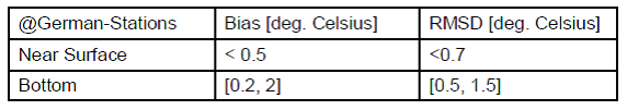
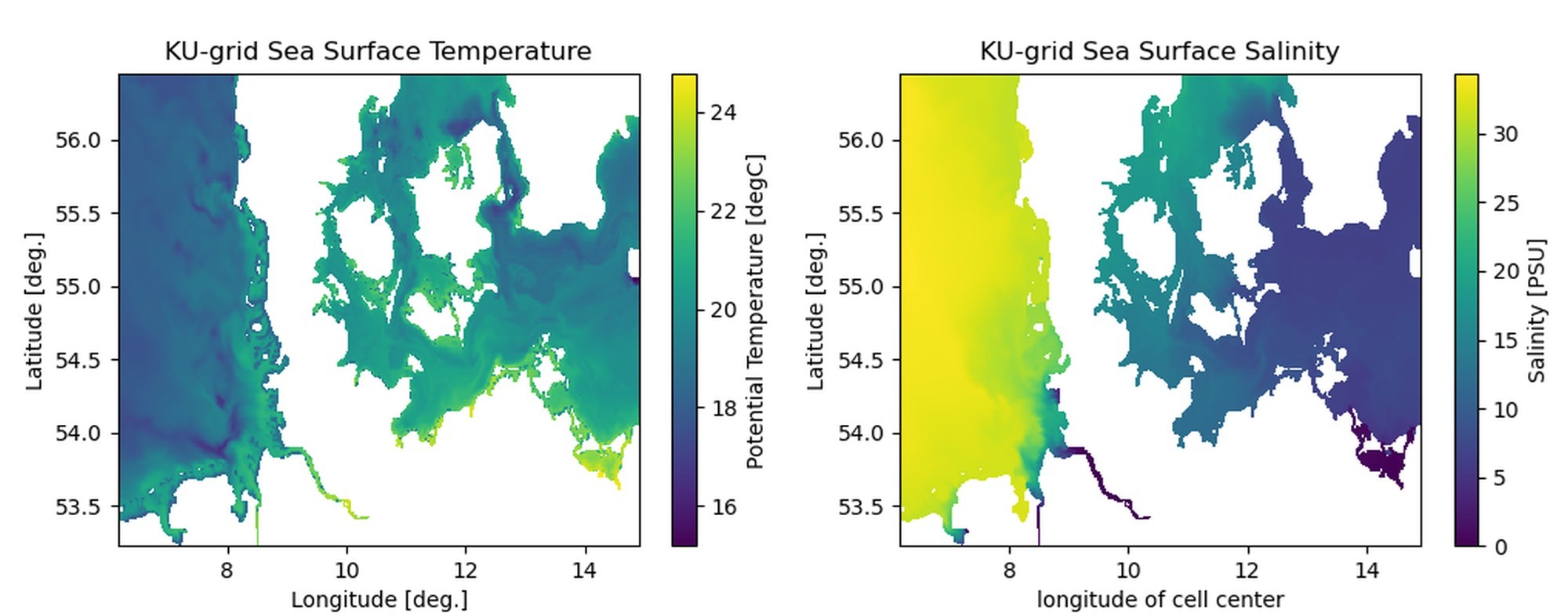
Since the early 1990s BSH operates and further enhances a baroclinic regional forecast model (Dick et al. 2001). The model consists of two two-way nested grids covering the entire North Sea and Baltic Sea from approx. 4° W to approx. 30° E and approx. 49.5° N to approx. 61° N (North Sea), respectively approx. 53° N to approx. 65.5° N (Baltic Sea). The finer grid covers the German coastal waters from approx. 6° E to approx. 15° E and approx.53° N to approx. 56.5° N (Figure 5). The current implementation of the model (BSHcmod) has a horizontal resolution of half a nautical mile (approx.900(m) and consists of up to 25 depth layers as either dynamic coordinates on the native model grid or interpolated to fixed z-coordinates on a so-called product grid. For this investigation, the product grid option was chosen due primarily to much simpler data handling. Since the surveyed datasets have a mean depth of approx. 19m, there are only five usable depth layers in the product grid: 0, 4, 9, 12 and 17 meters depth at which hourly forecasts of temperature and salinity are available. Atmospheric forcing is provided by the operational forecasts of the German Weather Service (DWD). At the open model boundaries, surge data and tides based on 19 partial constituents are used as well as monthly temperature and salinity data from Janssen, Schrum, and Backhaus (1999). BSHcmod demonstrated good agreement to measured temperate at German stations in the North Sea and Baltic Sea (Table 2). However, while the model captured the surface salinity and the permanent halocline in the Baltic Sea quite well, it was less accurate at other depths (Brüning et al. 2014).
Synthetic sound speed profiles were derived from BSHcmod using the dependencies on temperature, salinity and pressure on depth following Chen and Millero (1977) for every available sample location and time covering the spatial and temporal extent of the survey datasets.
2.3 Spatiotemporal Interpolation
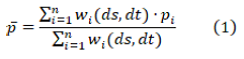
A spatialtemporal interpolation routine from Roemer et al. (2017) was used to generate synthetic sound speed profiles at any chosen location and time. The prediction routine is a distance (in both space and time) weighted deterministic interpolator where the sound speed profile at position and time  is the weighted sum of all other sound speed profiles
  :
:
where:
 is the distance-based weight for profile
  is the time-based weight for profile
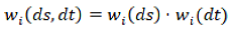
The weights and , where  represents the geodetic distance and the
  elapsed time (i.e. time distance) respectively between profile and the desired prediction at some spatial and time location , decreases exponentially as a function of distance according to:
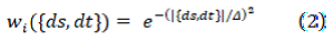
The parameter  controls the weight contribution
  of the observed profiles on the predicted profile and is determined from Equation (2) based on a user-specified weight contribution at a specific distance:
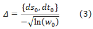
 and
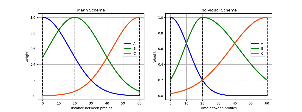
and  are determined either as the average minimum distance between all observed profiles (mean scheme) or the individual distances between observed profile pairs (individual scheme). While the weight contribution will be identical for a fixed distance in the mean scheme, the individual scheme allows for specific weight contributions for all observed profile pairs. Figure 6 illustrates how the mean and individual schemes work for the case of three hypothetical profiles.
As in any deterministic interpolation method, the difficulty resides in properly determining the weights. In this investigation, the weight contributions are handled differently for the spatial and temporal components. Based on initial recommendations from Roemer et al. (2017), the spatial weight contribution was determined using the mean scheme while the time weight contribution was determined using the individual scheme. This allows identical geodetic distance-based weight contributions and specific weight contributions forward and backward in time simultaneously. The desired weight contribution was fixed at 20%, representing a 20% contribution of any observed profile at the distance or determined according to the chosen scheme.
2.4 Ray-Tracing Techniques
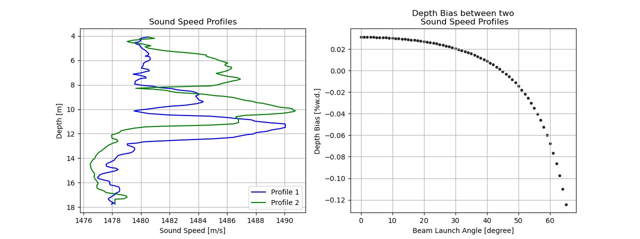
In order to quantify the depth accuracy of soundings ray-traced using synthetic profiles, a simulated ray-tracing approach was applied between profile pairs consisting of measured MVP-30 profiles and synthetic profiles. Beaudoin (2010) demonstrated how this approach can be used to quickly determine the vertical and horizontal biases between the differing ray-traced solutions of two different sound speed profiles without the need for any sounding data. Given a chosen reference depth and beam launch angle, the two-way travel time (TWTT) to reach that reference depth using the first profile is calculated. That same beam launch angle and TWTT is then applied with the second profile in order to obtain a second ray-traced solution. The differing ray-traced solutions between the two profiles is measurable as a vertical and horizontal bias in the ray-tracing plane and is indicative of the relative impact of using one profile versus the other for the determination of the 3D sounding position. Figure 7 illustrates the vertical relative bias (right plot) between two sound speed profiles (left plot) at one degree beam intervals for beam launch angles ranging from 0° to 70°. Note that the depth bias is 0, which is consistent with the type IV signature of a ray-tracing error.
In this investigation, a maximum allowable depth bias of 0.25% of water depth due solely to the ray-tracing error was fixed. This is a realistic requirement compatible with the uncertainty budget of the multibeam system. Indeed, the total depth uncertainty within the beam launch angles [−65°, 65°] is approx. 1% of depth (see Figure 1) and attributing 25% of the total depth uncertainty to the sound speed uncertainty is a reasonable and standard accepted practice.
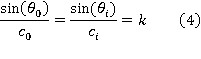
The ray-tracing function available in the software application Sound Speed Manager (Gallagher et al. 2017) is used to calculate the depth bias for a hypothetical 65° beam launch angle. In order to obtain realistic results, the transducer immersion depth was considered as the starting ray-tracing depth and the measured surface sound speed was also incorporated for all sound speed profile ray-tracing comparisons. Indeed, as described in Cartwright and Hughes Clarke (2002), merging the measured sound speed at the face of a flat array antenna with the sound speed profile leads to the addition of a snap-back layer which guarantees that the ray parameter in Equation (4) will be correctly determined based on the original beam launch angle
  and the measured surface sound speed
  and is valid for all subsequent layers
  (Tonchia and Bisquay 1996).
The ray-tracing function available in Teledyne-CARIS HIPS and SIPS (version 11.3) was also used to ray-trace the soundings of the multibeam datasets using both measured and synthetic profiles, thereby building the basis for direct sounding depth differences. This process was applied at the survey line level by exporting the soundings from HIPS in the GSF format and using the UKHO gsfpy library (UKHO 2021).
2.4 Fusion of Real and Synthetic Sound Speed Profiles
Once synthetic sound speed profiles can be derived using ancillary sources (Sections 2.2 and 2.3) and their relative impact on sounding depth accuracy evaluated (Section 2.4), the challenge mainly consists in optimally distributing them spatially and temporally. In theory, a synthetic profile can be derived at every infinitesimal azimuth dependent geodetic distance  within the survey area and every infinitesimal time interval within the survey duration. A foreseeable advantage of this method would be for those cases when the water column horizontal stratification assumption in current ray-tracing models were to prove unsuitable, such as when surveying under the presence of internal waves (Hamilton and Beaudoin 2010). If the assumption holds however, then a more appropriate practice consists in deriving a unique sound speed profile for every ping along each survey line (about every 80ms in 20m depth for a 140° swath opening). Even at this sampling period, it remains to be proven if this practice brings a benefit in terms of sounding positional accuracy or if it simply creates redundant data with little gain. Current spatial and temporal scales of regional forecast models such as BSHcmod (approx. 900m and hourly forecasts) are most likely too coarse to provide such benefits. Sound speed profile interpolation, on the other hand, is beneficial if the sound speed profile sampling period is chosen as to fully capture the spatiotemporal scale of the oceanographic processes as demonstrated by Hughes Clarke, Lamplugh, and Kammerer (2000) using a single 45km survey transect across George Banks (Canada). Inline with this approach, Figure 8 illustrates the vertical sound speed structure of survey dataset C (see Figure 3) using several combinations of measured and synthetic sound speed profiles. Figure 8a displays the water column as observed using the MVP-30 reference dataset with a sampling period of 2 min interpolated at a 1s period. The azimuth of the 16 survey lines is portrayed above the figure and is correlated with the change in sound speed in the deeper layers. The spatial scale of the observed sound speed is obviously directly related to the survey pattern. Given that the mean time of a single survey line is 19 minutes, only a sampling period of 19 minutes or less will capture the full spectrum of the water column in accordance with the Nyquist criterion (Proakis and Manolakis 1996). This is well illustrated in Figure 8b and Figure 8c where the same periodicity as Figure 8a is observable for sampling periods of 8 and 16 minutes respectively. On the contrary, Figure 8d, with a corresponding sampling period of 31 minutes, is strongly affected by aliasing.
Many hydrographic organizations utilize the direct comparison between the continuously measured sound speed at the transducer face and the sound speed value at the transducer immersion depth of the last measured profile to determine the profile sampling period (LINZ 2020; NOAA 2018). There are several drawbacks to this method:
- Only changes in the upper-layer of the water column are considered;
- The surface sound speed sensor needs to be error free;
- The fusion of the surface sound speed into the sound speed profile for ray-tracing will minimize the deviation between the last profile and current conditions in the upper-layer.
Point #1 is well illustrated in Figure 8, where the transducer immersion depth is illustrated as a dashed black line. During the complete survey, the surface sound speed remained within a 2m/s bound whereas the deeper layer showcased higher variability. A closer monitoring of the complete water column following, for example, the wedge analysis method proposed by Beaudoin (2010), offers more potential to detect such changes in the water column. Determining an appropriate sound speed profile sampling period would still require a higher measurement frequency at the start of the survey until the variability of the water column is well understood. An underway system can be envisioned in which the sampling period is automatically adjusted following a real-time analysis of the oceanographic variability. This analysis could consist in comparing the last measured sound speed profile with an optimal predicted profile of the sound speed variability ahead of the survey platform, derived from a spatiotemporal interpolation and a suitable regional forecast model. It is therefore essential to first establish the level of adequacy of synthetically derived sound speed profiles for use in hydrographic surveying. Section 3 addresses this level of adequacy in this investigation.
3. RESULTS AND DISCUSSION
Based on the data and techniques presented in the previous chapter, Section 3.1 attempts to assess the depth accuracy of synthetic sound speed profiles derived from BSHcmod. Using a similar procedure, Section 3.2 attempts to assess the depth accuracy of synthetic sound speed pro- files determined by interpolation from a subset of measured sound speed profiles. Both assessments use the MVP-30 dataset as reference. In Section 3.3, a relative assessment of the depth bias accuracy is performed, based on a flat-bottom assumption.
3.1 Absolute Accuracy of Regional Forecast Model
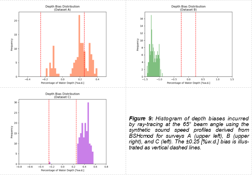
The absolute accuracy of synthetic sound speed profiles derived from BSHcmod was evaluated by comparing the ray-tracing solution of these profiles against the measured sound speed profiles from the MVP-30. The interpolator described in Section 2.3 was used to account for the exact location and time of each measured profile. Figure 4 illustrates the derived synthetic profiles (in brown) which can be qualitatively compared to the measured profiles (in black). Figure 9 illustrates the histogram distribution of depth biases computed by ray-tracing each profile pair (real versus synthetic) at the 65° beam angle. The mean transducer immersion depth and the measured sound speed at the transducer face were factored into the computation. For datasets B and C, the systematic error introduced by using the synthetic profiles is significant and would lead to the survey not meeting the maximum 0.25% depth bias requirement for depth uncertainty. In dataset A, BSHcmod somewhat better captures the sound speed variability on that particular survey day. Although the depth bias distribution is clearly not uniformly distributed, using the modeled profiles instead of the measured profiles would lead to the survey partially fulfilling the requirements for depth uncertainty. While both BSHcmod and the interpolator contributed to the creation of the synthetic profiles, it can be reasonably assumed from inspection of Figure 4 that the major bias contribution arises from BSHcmod itself.
3.2 Absolute Accuracy of Spatiotemporal Interpolation
In order to evaluate the accuracy and reliability of interpolation in compensating for the lack of measured sound speed profiles, five subsets (4T, 8T, 16T, 32T and 64T) with increasing sound speed profile sampling period were created by downsampling the full-resolution MVP-30 dataset. The sampling period is thereby increased from, for example for dataset C, a minimum mean period of 2 minutes (fundamental period T) to a maximum mean period of 128 minutes (64 times the fundamental period T). The profiles of each subset were then used as observations in the interpolation in order to derive synthetic profiles at the exact location and time of the measured MVP-30 profiles. The root-mean-square (RMS) deviation of the depth biases computed by ray-tracing using the procedure outlined in section 3.1 for all profile pairs (real versus synthetic) quantifies the error introduced by replacing real with synthetic profiles. The gain obtained by interpolation can further be assessed by calculating the RMS deviation without interpolation, i.e. by pairing each MVP-30 sound speed profile with its profile nearest in time within each subset. Table 3 summarizes the RMS deviations expressed as percentage of water depth for the three survey datasets A, B and C. The maximum RMS deviation across all datasets reaches 0.11%, corresponding to only 2 cm in 20 m depth. As expected, the RMS deviation generally increases as the number of measured profiles decreases. Dataset A showcases almost no gain from interpolation, which is consistent with the low sound speed variability on that survey day. Datasets B and C showcase a maximum gain from interpolation of only 0.04%, corresponding to 1 cm in 20 m water depth.
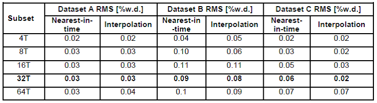
With a mean sampling period of 83 min and an average number of sound speed profiles of seven across all datasets, subset 32T best approximates current survey practices at BSH. It is therefore retained in order to evaluate more closely the distribution of depth biases. Figure 10 presents the distributions of depth biases for subset 32T. The results are consistent with the observations made in Table 3. Indeed, aside from an outlier in dataset B, all other depth biases remain within the 0.25% maximum depth bias requirement. For datasets A and B, interpolation slightly reduces the depth bias. For the dataset C, where the distribution of depth biases was not centered about the zero bias, interpolation also recenters the depth bias distribution about zero. This helps to explain why the best results are obtained for dataset C.
In order to evaluate how significant the profile selection is in the depth distribution, a second method of selection was tested across all datasets. In this method, the seven sound speed profiles that optimize the mean distance between profile locations are retained. Figure 11 presents the histograms of depth biases using this profile selection method. The effect of the interpolation is very similar to the time-ordered downsampling method whose results were presented in Figure 10. The effect of the profile selection between time and distance can therefore empirically be assumed to be benign.
The effectiveness of the interpolation was further evaluated on real multibeam measurements. Figure 12 illustrates the depth bias as a function of beam launch angle for a single survey line handpicked from each survey dataset A, B and C. In each case, the survey line corresponding to the worst affected part of the bathymetric model was chosen. The red curves were obtained by subtracting the soundings ray-traced using the full MVP-30 sound speed profiles to those ray- traced using subset 32T (Nearest-in-time) (ref. Table 3) and the blue curves were obtained by subtracting the soundings ray-traced using the full MVP-30 sound speed profiles to those ray- traced using subset 32T (Interpolation). In all cases, the depth bias is zero at the beam launch angle, which is consistent with the signature of a type IV ray-tracing error. Figure 13 presents the mean bias and standard deviation computed from the bias curves in Figure 12. Clearly, interpolation provides a benefit in terms of depth bias and spread reduction across the swath for datasets B and C, the benefit being more noticeable in the outer parts of the multibeam swath (e.g. a factor three reduction in the mean depth bias for dataset B at the -70° beam angle). Interestingly for dataset A, where survey conditions were very stable, interpolation leads to an over- compensation of the mean bias and a small worsening of the spread.
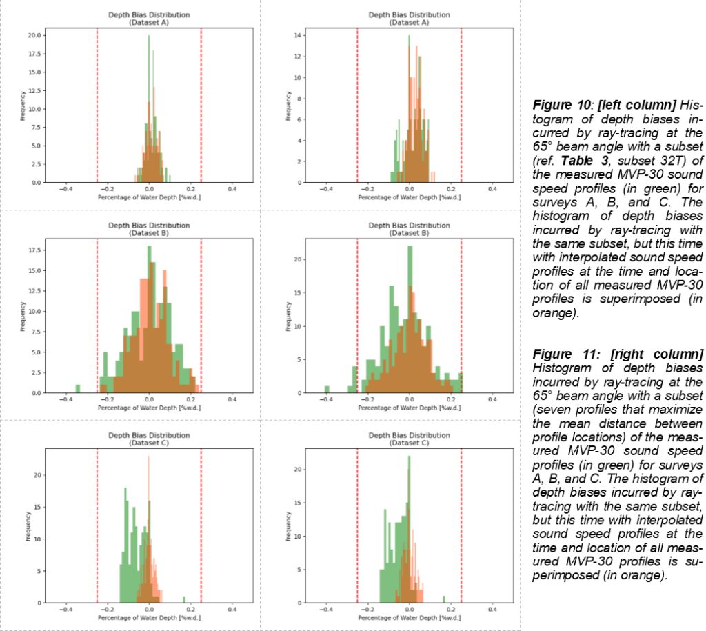
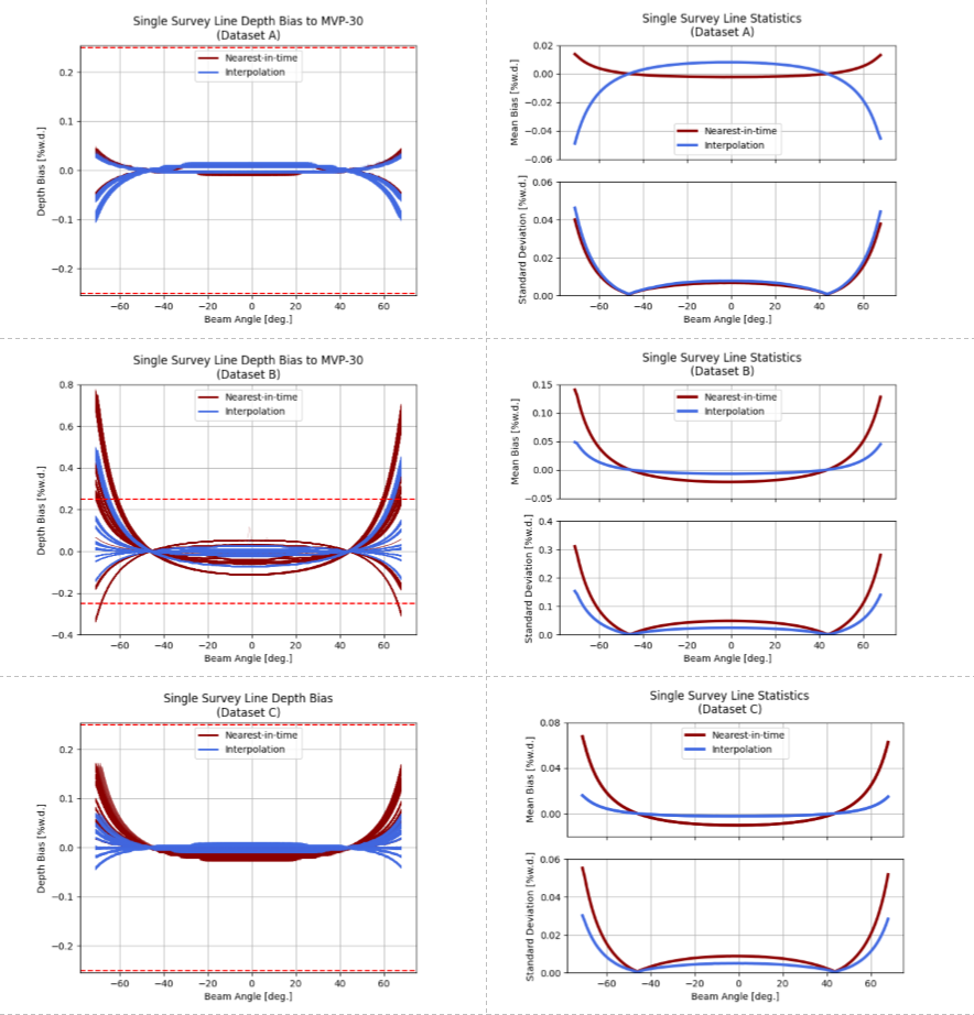
Figure 13: [right column] Mean depth bias and standard deviation computed from the depth biases in Figure 12. Note that the plots do not share the same vertical scale.
3.3 Relative Accuracy of Residual Depth Bias
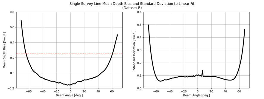
The depth bias incurred by a reduction of the number of measured sound speed profiles from a full resolution MVP-30 dataset is significant, but remains relatively small in comparison to the depth biases observable on control lines (see for example Figure 1). Therefore, a linear regression was performed on each swath of the survey lines displayed in Figure 12 in order to quantify the depth bias of the full resolution MVP-30 dataset compared to a flat-bottom assumption. The resulting mean depth bias and standard deviation for dataset B are plotted in Figure 14. The angle dependent signature of the mean bias is again reminiscent of a type IV error, but is likely not due to a ray-tracing error given the small mean profile sampling period of 2.3 min. The magnitude of the mean bias is significant (0.25% of depth at a beam angle of -60°, corresponding to 5 cm in 20 m depth; see Figure 14, left) and is most likely not due to the natural bottom topography, which is implicit in the mean bias curve due to the simplified flat bottom assumption. Figure 14 (right) points towards a bottom topography that certainly does not exceed 0.1% of water depth. It is therefore hypothesized that a beam steering error rather than a ray-tracing error dominates the sound speed error contribution in the datasets presented. Given that the surface sound speed sensor is subjected to a regular maintenance and calibration schedule, it is unlikely that a factory calibration would resolve the issue.
4. SUMMARY AND OUTLOOK
Synthetic sound speed profiles were derived from the BSHcmod regional forecast model and were compared to measured profiles using a simulated ray-tracing approach. Results indicated that the depth bias incurred with synthetic profiles exceeds the 0.25% maximum allowable depth bias. Combining real with model-based profiles would therefore likely be detrimental to the overall bathymetric accuracy. However, BSHcmod has been in operational use since the early 1990s and was in the process of being renewed as this investigation took place. In early 2021, a new imple- mentation of the BSH regional forecast model was released, now called BSH-HBM. BSH-HBM enhances BSHcmod by increasing the depth resolution and improving the quality of the forecast data. Temperature and salinity forecasts are available in two meter increments for the upper 20 meters and Sea Surface Temperature (SST) data are now being assimilated (Brüning et al. 2014; Brüning et al. 2021). In the near future, temperature and salinity forecasts will also be assimilated. These enhancements should significantly improve the quality of forecasts and thus the potential of using this new iteration for survey purposes. Parallel to BSH-HBM, a higher-resolution (< ap- prox. 200m) regional hydrodynamic model from the Leibniz Institute for Baltic Sea Research, Warnemünde (IOW), is also currently under investigation (Burchard and Bolding 2002; Klingbeil and Burchard 2013).
A spatiotemporal deterministic interpolator demonstrated effectiveness at reducing the mean and spread of depth biases. The choice of sound speed profiles subsampling method, i.e. time or location based, did not influence at first sight the results, but this should be proven statistically. The added-value of interpolation is small, but nevertheless significant. The gain in depth accuracy is a function of the water column variability in time and space as well as on the sampling period. In all cases, an increase in the usable portion of the multibeam swath is potentially achievable. A single set of parameters were used for the interpolation. Further parametrizing is possible and could be attempted to balance the time and spatial weight distribution. An objective method to determine these weights from the regional forecast models could be based on geostatistical techniques.
Residual type IV depth biases observable in the reference datasets lead to a requestioning of the original hypothesis that the ray-tracing error is the dominant sound speed error source. A beam steering error due to an incorrect surface sound speed value is considered as a possibly more significant source of error. One way to validate this hypothesis would be to look for characteristic type III errors in the datasets. Indeed, since the beam steering error is array relative, its signature in the geographic frame will be distorted by the rolling motion of the ship and a characteristic type III error should be visible. The detection of this error signature will solidify the hypothesis of a beam steering error and may be achievable in the method described by Maingot, Hughes Clarke, and Calder (2019).
5. CONCLUSION
An approach to combine real and synthetic sound speed profiles derived from either a regional forecast model or spatiotemporal interpolation was presented. The motivation stems from a desire to mitigate the effect of sound speed errors on multibeam measurements. Results indicated that the model used in this investigation (BSHcmod) leads to significant depth biases when applied for hydrographic operations. Interpolation provides a benefit in terms of increased swath with up to a factor three depth bias reduction at higher beam angles. During the analysis, a possible beam steering error was identified as being a significant contributor to the sounding depth uncertainty. Using the proposed approach, and provided that the source of the beam steering error can be mitigated, the accuracy of multibeam data in German coastal waters will be significantly increase.
6. ACKNOWLEDGMENTS
The authors would like to address their sincere appreciation to Mr. Swen Roemer for the insightful suggestions and many contributions to the spatiotemporal interpolator.
7. DATA AVAILABILITY STATEMENT
The data that support the findings of this study are available from the corresponding author, Jean-Guy Nistad, upon reasonable request.
8. REFERENCES
– Beaudoin, J., J. E. Hughes Clarke, and J. Bartlett. 2006. “Usage of Oceanographic Databases in Support of Multibeam Mapping Operations Onboard the CCGS Amundsen.” Lighthouse, Journal of the Canadian Hydrographic Association Edition No. 68.
– Beaudoin, Jonathan. 2010. “Real-time Monitoring of Uncertainty due to Refraction in Multibeam Echo Sounding.” The Hydrographic Journal 134:3-13.
– Brüning, Thorger, Frank Janssen, Eckhard Kleine, Hartmut Komo, Silvia Maßmann, Inge Menzenhauer-Schuhmacher, Simon Jandt, and Stefan Dick. 2014. “Operational Ocean Forecasting for German Coastal Waters.” Die Küste 81:273-90.
– Brüning, Thorger, Xin Li, Fabian Schwichtenberg, and Ina Lorkowski. 2021. “An operational, assimilative model system for hydrodynamic and biogeochemical applications for German coastal waters.” Hydrographische Nachrichten – Journal of Applied Hydrography 118:6-15.
– Burchard, Hans, and Karsten Bolding. 2002. “GETM, A General Estuarine Transport Model, Scientific Documentation.” Technical Report EUR 20253 EN, Eur. Comm. Leibniz-Institut für Ostseeforschung Warnemünde.
– Calder, Brian R., Barbara J. Kraft, Christian de Moustier, J. Lewis, and P. Stein. 2004. Model- based Refraction Correction in Intermediate Depth Multibeam Echosounder Survey. Paper pre sented at the Proceedings of the European Conference on Underwater Acoustics (ECUA), 2004/july 5 – 8.
– Capell, William J. 1999. Determination of sound velocity profile errors using multibeam data. Paper presented at the Oceans ’99. MTS/IEEE. Riding the Crest into the 21st Century. Conference and Exhibition. Conference Proceedings (IEEE Cat. No.99CH37008), 1999.
– Cartwright, D. S., and J. E. Hughes Clarke. 2002. Multibeam surveys of the Frazer river delta, coping with an extreme refraction environment. Paper presented at the Proceedings of the Canadian Hydrographic Conference, 2002/05.
– Chen, C. T., and F. J. Millero. 1977. “Speed of sound in seawater at high pressures.” Journal of the Acoustical Society of America 62:1129-35.
– Church, Ian William. 2020. “Multibeam Sonar Ray-Tracing Uncertainty Evaluation from a Hydrodynamic Model in a Highly Stratified Estuary.” Marine Geodesy:1-17.
– Dehling, Thomas, and Wilfried Ellmer. 2012. “Zwanzig Jahre Seevermessung seit der Wiedervereinigung.” AVN 119 (7).
– Dick, Stephan, Eckhard Kleine, Sylvin H. Müller-Navarra, Holger Klein, and Hartmut Komo. 2001. “The Operational Circulation Model of BSH (BSHcmod).” Technical Report 29. Bundesamt für Seeschifffahrt und Hydrographie.
– Ding, Jisheng, Xinghua Zhou, and Qiuhua Tang. 2008. “A method for the removal of ray refraction effects in multibeam echo sounder systems.” Journal of Ocean University of China 7 (2):233-6.
– Dinn, Donald F., Bosko D. Loncarevic, and Gerard Costello. 1995. The effect of sound velocity errors on multi-beam sonar depth accuracy. Paper presented at the ‘Challenges of Our Changing Global Environment’. Conference Proceedings. OCEANS ’95 MTS/IEEE, 1995.
– Eeg, Joergen. 1999. “Towards Adequate Multibeam Echosounders for Hydrography.” International Hydrographic Review 76 (1):33-48.
– Eeg, Joergen. 2010. “Multibeam Crosscheck Analysis – A Case Study.” International Hydrographic Review 10 (4):25-33.
– Gallagher, B., G. Masetti, C. Zhang, B. R. Calder, and M. Wilson. 2017. Sound Speed Manager: An Open-Source Initiative to Streamline the Hydrographic Data Acquisition Workflow. Paper presented at the Proceedings of the U.S. Hydro Conference, 2017/march 20-23.
– Hamilton, Travis, and Jonathan Beaudoin. 2010. “Modelling Uncertainty Caused by Interval Waves on the Accuracy of MBES.” The International Hydrographic Review 13 (4).
– Hengl, Tomislav. 2009. A Practical Guide to Geostatistical Mapping: European Commission, Joint Research Centre, Institute for Environment and Sustainability.
– Hughes Clarke, John E. 2003. “Dynamic Motion Residuals in Swath Sonar Data : Ironing out the Creases.” International Hydrographic Review 4 (1):6-23.
– Hughes Clarke, John E., Mike Lamplugh, and Edouard Kammerer. 2000. Integration of near- continuous sound speed profile information. Paper presented at the Proceedings of the Canadian Hydrographic Conference, 2000/16-18 may.
– IHO. 2020. “International Hydrographic Organisation Standards for Hydrographic Surveys.” Publication S-44. Edition 6.0.0.
– Janssen, Frank, Corinna Schrum, and J. Backhaus. 1999. “A climatological data set of temperature and salinity for the Baltic Sea and the North Sea.” Deutsche Hydrographische Zeitschrift 51:5-245.
– Kammerer, Edouard, and John E. Hughes Clarke. 2000. New method for the removal of refraction artifacts in multibeam echosounder systems. Paper presented at the Proceedings of the Canadian Hydrographic Conference, 2000/16-18 may.
– Klingbeil, Knut, and Hans Burchard. 2013. “Implementation of a direct nonhydrostatic pressure gradient discretisation into a layered ocean model.” Ocean Modelling 65:64-77.
– LINZ. 2020. “HYSPEC – Contract Specifications for Hydrographic Surveys Version 2.0.” New Zealand Hydrographic Authority.
– Maingot, B., J. E. Hughes Clarke, and B. Calder. 2019. High Frequency Motion Residuals in Multibeam Data: Identification and Estimation. Paper presented at the Proceedings of the U.S. Hydrographic Conference, 2019/19-21 march.
– Masetti, Giuseppe, Michael J. Smith, Larry A. Mayer, and John G. W. Kelley. 2020. “Applications of the Gulf of Maine Operational Forecast System to Enhance Spatio-Temporal Oceanographic Awareness for Ocean Mapping.” Frontiers in Marine Science 6:804-.
– Mohammadloo, T. H., M. Snellen, W. Renoud, J. Beaudoin, and D. G. Simons. 2019. “Correcting Multibeam Echosounder Bathymetric Measurements for Errors Induced by Inaccurate Water Column Sound Speeds.” IEEE Access 7:122052-68.
– NOAA. 2018. “NOS Hydrographic Surveys Specifications And Deliverables.” National Oceanic and Atmospheric Administration U.S. Department of Commerce, National Ocean Service.
– North, Ryan P., and David M. Livingstone. 2013. “Comparison of linear and cubic spline methods of interpolating lake water column profiles.” Limnology and Oceanography: Methods 11 (4):213-24.
– Peyton, Derrick R., Jonathan Beaudoin, and Michael Lamplugh. 2009. “Optimizing Sound Speed Profiling for Hydrographic Surveys.” The International Hydrographic Review 9 (2).
– Proakis, John G., and Dimitris G. Manolakis. 1996. Digital Signal Processing (3rd Ed.): Principles, Algorithms, and Applications: Prentice-Hall, Inc.
– Ridgway, K. R., J. R. Dunn, and J. L. Wilkin. 2002. “Ocean interpolation by four-dimensional weighted least squares—Application to the waters around Australasia.” Journal of atmospheric and oceanic technology 19 (9):1357-75.
– Riecken, Jens, and Enrico Kurtenbach. 2017. “Der Satellitenpositionierungsdienst der deutschen Landesvermessung–SAPOS®.” Zeitschrift für Geodäsie, Geoinformation und Landmanagement (ZfV) 142 (5):293–300-293–300.
– Roemer, S., D. A. Hodnesdal, A. E. Ofstad, and A. F. Dias. 2017. Sound velocity profile interpolation in space and time – a way to overcome one of the nightmares of multi-beam processing? Paper presented at the Teledyne CARIS International User Group Conference, 2017/19-22 june.
– SAPOS. 2021. “Satellitenpositionierungsdienst der Deutschen Landesvermessung.” Accessed 24/08/2021. https://sapos.de/.
– Tollefsen, Cristina, and Sean Pecknold. 2010. “Comparison of Sound Speed Profile Interpolation Methods with Measured Profiles; Effects on Modelled and Measured Transmission Loss.” Canadian Acoustics 38 (3):60-1.
– Tonchia, Hélène, and Hervé Bisquay. 1996. The effect of sound velocity on wide swath multibeam system data. Paper presented at the OCEANS 96 MTS/IEEE Conference Proceedings. The Coastal Ocean – Prospects for the 21st Century, 1996.
– UKHO. 2021. “gsfpy – Generic Sensor Format for Python.” Accessed 08/04/2021. https://github.com/UKHO/gsfpy.
– Yang, Fanlin, Jiabiao Li, Ziyin Wu, Xianglong Jin, Fengyou Chu, and Zhongzhi Kang. 2007. “A post-processing method for the removal of refraction artifacts in multibeam bathymetry data.” Marine Geodesy 30 (3):235-47.
9. AUTHORS BIOGRAPHIES
Jean-Guy Nistad hold s an engineering degree from McGill University (Canada), a graduate diploma in GIS from Université du Québec à Montréal and a graduate degree in hydrography completed at the HafenCity University Hamburg, recognized as a FIG/IHO Cat. A. educational program. From 2007 to 2013 he worked for CIDCO (Canada) where he gained most of his expertise in hydrographic surveying. Since 2016, he has been employed by BSH, the Federal Maritime and Hydrographic Agency of Germany, in the section “Geodetic-hydrographic Techniques and Systems”. His current tasks include research & development, technical support on multibeam issues and hydrographic teaching.
Dr.-Ing. Patrick Westfeld graduated as a geodesist in 2005 from TU Dresden (Germany). He conducted research in the fields of photogrammetry and laser scanning and completed his PhD in 2012 on geometric-stochastic modeling and motion analysis. Since 2017, Dr. Westfeld heads the R&D section “Geodetic-hydrographic Techniques and Systems” at BSH, the Federal Maritime and Hydrographic Agency of Germany. The activities of his section range from conceptual issues pertaining to hydroacoustic and imaging sensor technologies, sensor integration and modeling, algorithmic development up to application-specific implementation and practical transfer in the production environment