

Abstract
1 Introduction
The international shipping industry, which contributed about 2.89 % of global Greenhouse Gas (GHG) emissions in 2018, has been urged to energy efficient operations of ships to address global climate change (Dewan & Godina, 2023). Ships with a gross tonnage (G/T) of 400 and above, built on or after January 1, 2013, are required to comply with the Energy Efficiency Design Index (EEDI) as per Regulation 24 of Annex 6 of the International Convention for the Prevention of Pollution from Ships (MARPOL). Ship built before January 1, 2013, have been subject to the Energy Efficiency Existing Ship Index (EEXI), a legal control similar to the EEDI, since November 1, 2022, in accordance with Regulation 25 of Annex 6 of MARPOL. Further, Regulation 28 of the Convention requires an operational Carbon Intensity Indicator (CII), a new measure for reducing GHG emissions, to be applied to ships of 5,000 G/T and above, regardless of their build date, starting from 2023 (IMO, 2021a).
The annual CII of individual ships is calculated as the ratio of the total mass of CO2 emitted to the total transport work undertaken in a given calendar year. The total mass of CO2 is equivalent to the sum of CO2 emissions from all the fuel oil consumed during the specific year. The annual CII of individual ships is categorized into five ratings, i.e. rating A, B, C, D or E which indicates a major superior, minor superior, moderate, minor inferior or inferior performance levels, respectively. It was analyzed that around 37.3 % of 684 ships registered in the Republic of Korea fell under ratings A and B, while about 34.2 % fell into the ratings D and E (Kim & Won, 2022). Another sample study on 140 ships, over 800 voyages calling at the South Asian ports between January 2021 and January 2022 showed that 34 % of the ships would have a non-compliant rating of CII in 2023 and it would rise to around 52 % of the ships in 2026 (Directorate General of Shipping, 2022). If a ship is rated as D of CII for three consecutive years or rated as E, it must submit its revised Ship Energy Efficiency Management Plan (SEEMP) to its Administration and take corrective actions to improve its CII level. Therefore, each vessel should consider how to maintain and improve a fair CII level. This implies that the ship is eager to save fuel oil to transport a cargo per mile. In other words, sailing longer distances with the same amount of fuel oil results in a better CII rating.
While new technologies such as hull air lubrication, automated fuel ejection timing systems, and energy recovery devices have been adopted to achieve a better EEDI (Rehmatulla & Tristan, 2020), several approaches of the operational measure like slow steaming, trim adjustment, route optimization, hull fouling removal and just-in-time operation in ports are being considered to improve the CII rating and EEXI by consuming less fuel oil (ICCT, 2021). The shipping industry should consider how to meet the CII rating requirements by implementing practical and efficient options to increase the energy efficiency of its fleet.
The energy efficiency of a ship can be simply defined by the distance a vessel travels with a given amount of fuel. Given that a ship propels itself using energy primarily generated by an internal combustion engine and sails at sea, both internal and external factors can affect the ship’s energy efficiency. The internal factors are related to the ship’s characteristics, including hull design, engine and propulsion efficiency. On the other hand, external factors that influence energy efficiency, particularly in coastal regions, include natural forces such as winds, waves, and tidal currents. If the external forces become significantly stronger in an adverse manner, the energy efficiency of a ship might gradually deteriorate under such conditions, as the amount of energy loss is likely to increase.
Natural forces, such as wind and tidal currents, have been harnessed for over a millennium to propel ships (Whitewright, 2018). Distinct from wind, tidal currents are characterized by their long-term predictability and relative insusceptibility to seasonal and global climatic variations (Byun et al., 2013). Tidal current velocity is significantly changed by the topography of the seabed and spring-neap tidal cycles. Consequently, the speed of a ship operating in coastal waters can be temporally and spatially influenced by tidal currents, thereby affecting the ship’s fuel consumption and energy efficiency. Navigation under favorable conditions yields superior economic and energy efficiency compared to navigation under adverse conditions (Casson, 1951).
Numerous studies have focused on speed optimization for the purpose of fuel conservation and reduction of energy consumption (Degiuli et al., 2021; Yang et al., 2020; Yu et al., 2019; Fagerholt et al., 2010; Corbett et al., 2009). Several approaches have investigated the impact of voyage optimization at the operational level on the reduction of greenhouse gas (GHG) emissions (Du et al., 2021; Wang et al., 2021; Safaei et al., 2019; Zaccone et al., 2018; Lu et al., 2015; Prpic-Oršic et al., 2014). However, it is evident that these studies primarily concentrate on the speed control of ocean-navigating vessels, which have additional operational options such as weather routing, trim/draft optimization, and arrival time adjustment to mitigate GHG emissions (Klakeel et al., 2023). These operational options, however, are unlikely to be selected for coastal shipping due to the constraints of limited alternative sailing routes and short distances that do not permit significant differentials from the options. Therefore, coastal shipping may need to explore other operational measures.
Considering that coastal regions are more consistently and predictably affected by tidal currents compared to external variables, this study aims to investigate the effect of tidal currents on the sailing speed of ships and their energy efficiency. In particular, we scrutinize these effects under different departure times within the tidal regime of the Korean coast (Fig. 1). For this analysis, we employ the Numerical Tidal Current Software (NTICS), developed by the Korea Hydrographic and Oceanographic Agency (KHOA), in tandem with actual performance data from a ship navigating between Yeosu Port and Incheon Port. Throughout this study, this software will be referred to as KHOA-NTICS.

2 Characteristics of tides and tidal currents
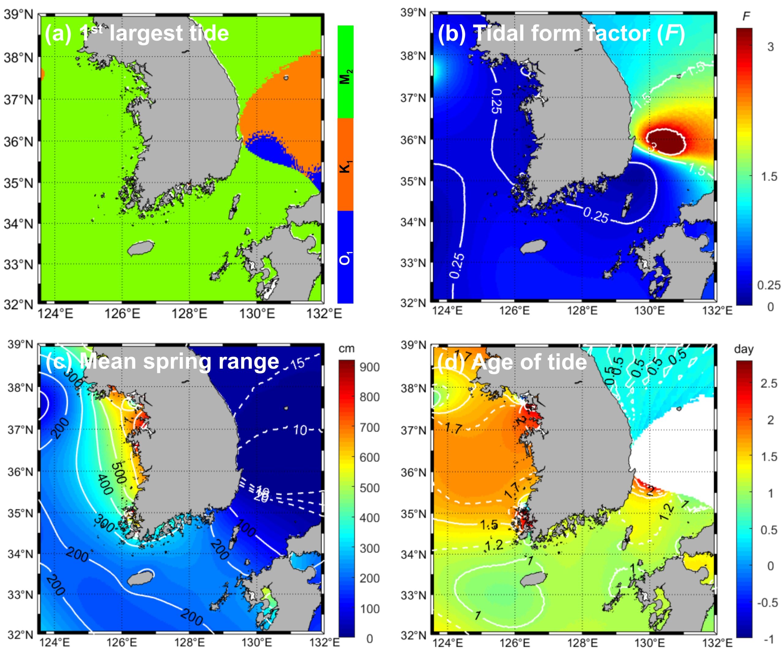
The west and south coasts of Korea are characterized by the M2-predominated semidiurnal tidal regime (Figs. 2a and 2b), showing different tide and tidal current characteristics. The mean spring tidal ranges (yielded as twice the sum of the M2 and S2 amplitudes) vary between 300 cm and 800 cm on the west coast but between 100 cm and 400 cm on the south coast of Korea (Fig. 2c). It is noteworthy that, in addition to these distinct tidal ranges, the west and south coasts also exhibit different degrees of spring retardation, also referred to as the age of the tide (calculated from the difference in phase lag, divided by the difference in angular speed between the S2 and M2 tides; Fig. 2d): the west coastal water shows higher delay values (>2 days), while the south coastal water exhibits lower delay values (ranging between >1 day and <1.5 days).
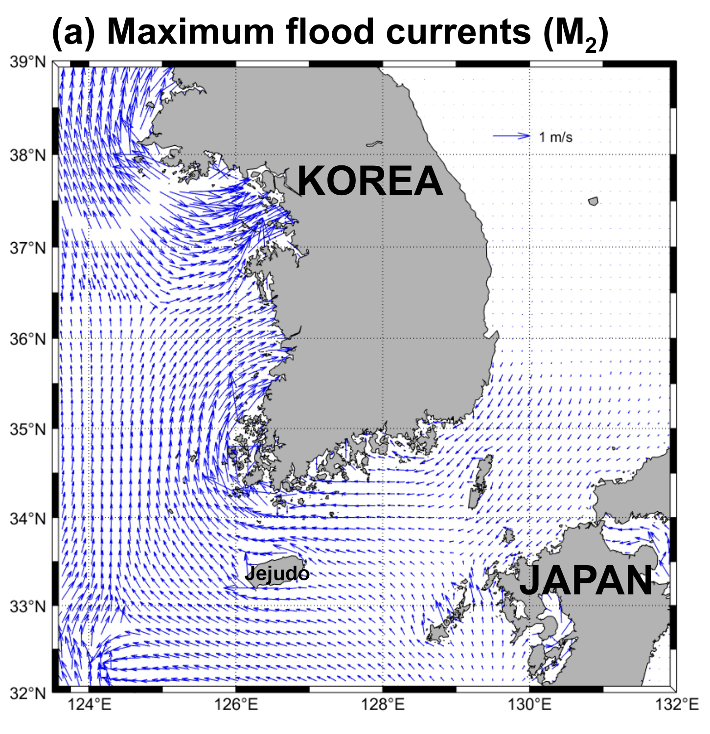
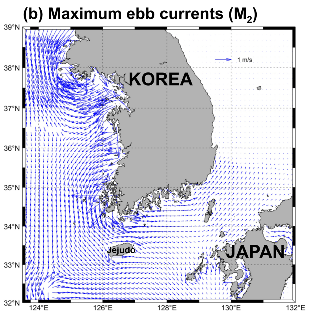
Compared to tides, tidal currents are more significantly influenced by bathymetry, including narrow waterways (Byun et al., 2013). Greater tidal ranges are observed in Gyeonggi Bay (>900 cm) on the west coast, while stronger (>4 m/s) tidal currents are present off the western tip of southwest Korea. The maximum flood currents in coastal areas are generally observed to flow towards the Korean Peninsula with a clockwise rotation during flood tides (Fig. 3a). In contrast, the maximum ebb currents tend to flow away from the Korean Peninsula with an anticlockwise rotation during ebb tides (Fig. 3b). More specifically, within the regional area, the flood (ebb) currents in the Korea Strait are inclined to flow from east (west) to west (east). Conversely, on the west coast of Korea, they flow towards (away from) the west of the Korean Peninsula (Fig. 3).
3 Methodology
3.1 Tidal current prediction using harmonic constants
Numerical models are commonly used worldwide to understand the characteristics of tidal regimes (Byun et al., 2004; Song et al., 2013) and to predict tides and tidal currents (Blain et al., 2002; Byun & Cho, 2009; Byun & Hart, 2022). Further, harmonic analyses of simulated tidal elevation and tidal-current results are used to produce information on the tidal constants (amplitudes and phase-lags) and tidal ellipse parameters (semi-major and semi-minor axes, inclination and phase) for the harmonic constituents. This information can be employed, in turn, in tide and tidal-current predicting and hindcasting through their prediction algorithms (Byun et al., 2023). Examples include the Polpred Offshore Tidal Software and Poltips Coastal Tidal Software programs developed by NOC (National Oceanography Centre Laboratory), and NTICS of KHOA, which are tide and tidal current prediction and visualization software. KHOA-NTICS has 16 tidal harmonic constant (M2, S2, K2, N2, L2, 2N2, T2, Mu2 and Nu2 for semidiurnal tides and K1, O1, P1, Q1, OO1, J1 and M1 for diurnal tides) database of three different horizontal resolutions of 250 m for Korean coastal water, and 500 m and 1 km for the Yellow Sea and Korea Strait in surface, middle and bottom layers. This study used the surface layer database of 500 m. Since 2006 (Kwon & Kang, 2007), this software has been gradually renovated.
Tidal current velocity C (=U+iV) can be predicted using harmonic constants for the easterly U and northerly V velocity components or their tidal ellipse parameters. Each component of tidal current velocity can be expressed by Byun & Hart (2017):
 |
(1) |
 |
(2) |
where the subscript k denotes each tidal current constituent; n is the total number of tidal current constituents; Vk is the astronomical arguments; (uu)k and (vv)k are the tidal harmonic constituent amplitudes and (gu)k and (gv)k are local time phase lags for u– and v-velocities components, respectively; ωk is the angular frequency; τ (=t0+t) is the reference time t0 plus the t elapsed since t0; ϕk is the phase of the maximum current; Φk is the inclination of the semi-major axis, measured anticlockwise from the x-axis; and fk and uk are the nodal amplitude factors and the nodal angles for the 18.61-year nodal modulation correction, respectively.
3.2 Calculating actual sailing distance
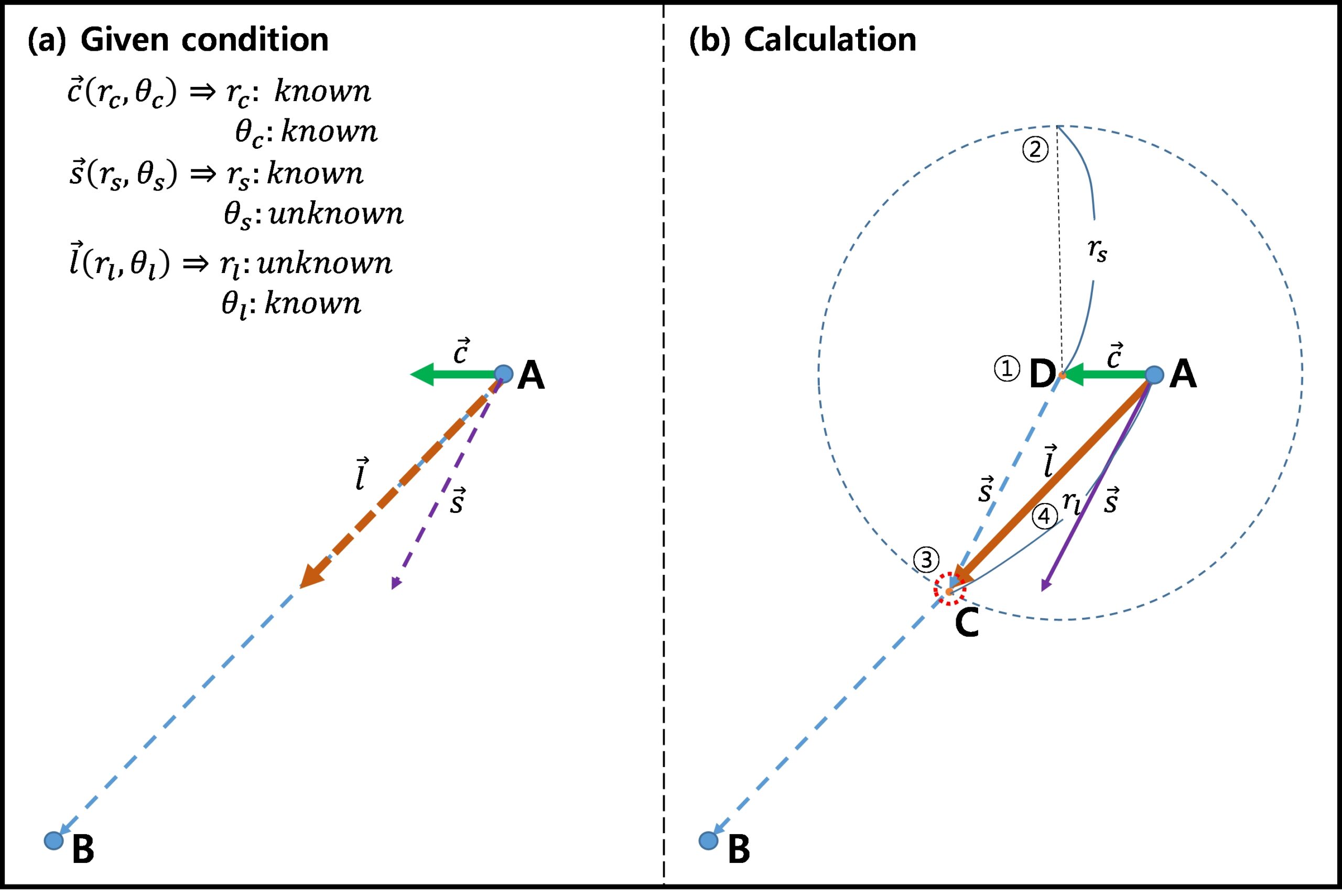
KHOA-NTICS, a tidal current prediction software based on a numerical model-derived harmonic constants, incorporates a feature that computes the anticipated arrival time along a chosen sailing route. This calculation takes into account the ship’s departure time and varying tidal current velocity fields. Under the conditions that tidal current velocity 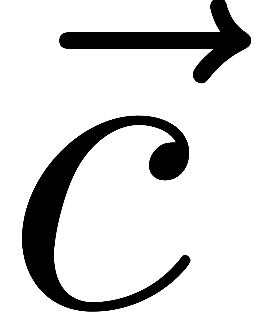 field and a ship speed
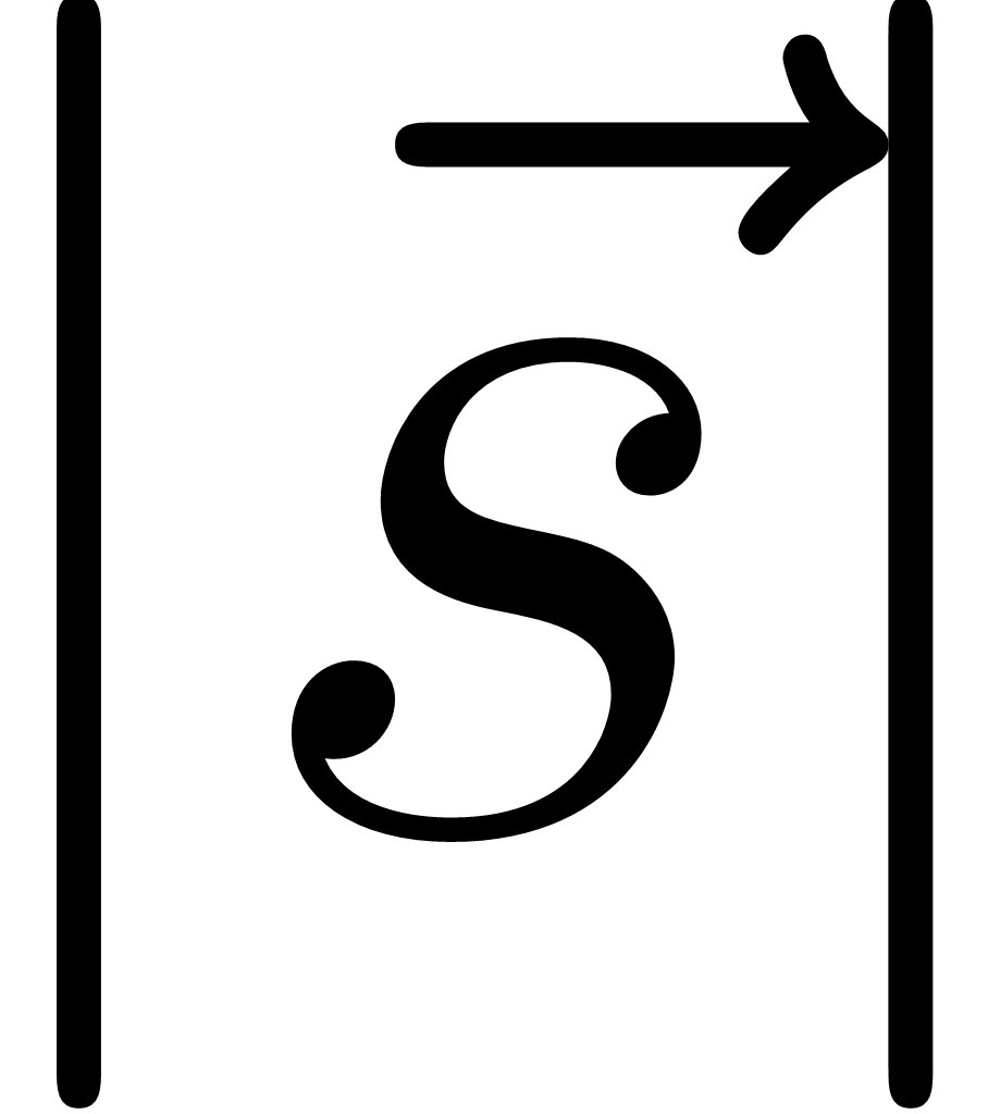 or rs are given and actual ship’s sailing direction
 is known (Fig. 4a), actual ship sailing speed rl on the given route in a certain time Δ t from point A can be calcuated as shown in Fig. 4b. The displacement of point D from point A is determined by the product of and Δt. Unknown
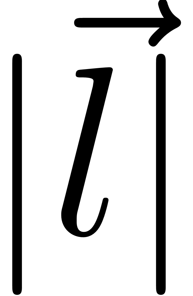 or rl is yielded by finding intersection point C between straight line
 and a circle with radius rl at point D (Fig. 4b). Distance vectors for each velocity in a certain time are expressed as
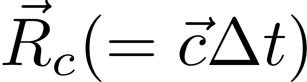 for tidal current velocity,
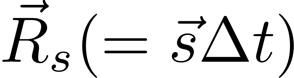 for ship velocity
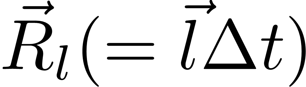 , and
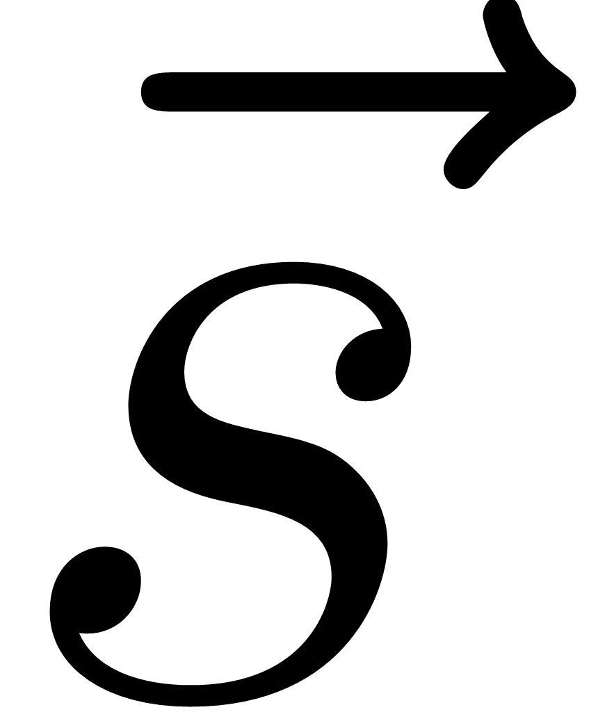 for actual ship velocity
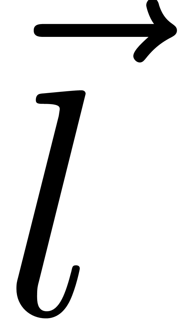 .
3.3 Experiment setting
In tidally dominated coastal environments, the ship’s speed is significantly influenced by the velocity of tidal current and the relative direction between the tidal current and the ship’s heading. The effect of tidal currents on a ship’s speed along Korea’s west and south coasts was analysed for spring (13–14 August 2022) and neap (20–21 August 2022) tidal periods using KHOA-NTICS. For this experiment, the sailing route is determined with selected 25 waypoints from Busan Port to Incheon Port, two major ports located on the southeast coast and west coast in Korea, respectively (Fig. 5). This sailing course, spanning a distance of 744 km (402 NM), was selected to draw waypoints to observe traffic separation schemes. The schemes were designed to reduce the likelihood of encountering reciprocal courses or crossing ahead of other vessel in area of heavy traffic, and to ensure safe passage by avoiding dangerous waters such as islands and rocks. In this study, we assumed a ship’s sailing speed in still water (absent the influence of tidal currents) to be 12.0 knots. By using KHOA-NTICS with the still water option, the travel time for the designated route is estimated to be 35 hr and 40 min.
Considering the variation in the tidal current velocity field at 10-minute intervals as provide by KHOANTICS, the experiments were primarily designed so that a vessel departs from the Busan Port at hourly intervals, starting from the high tide of the day. A fundamental procedure of calculating actual sailing distance in a changing tidal current velocity field is illustrated in Fig. 4. The actual tidal effect on a ship’s headway can be calculated from the composition of two vectors, i.e. the speed and direction of a ship in still water, and the corresponding direction and speed of the tidal current.
A vessel that sails with a tidal current experiences an increase in speed, while a ship that sails against the current experiences a reduction in headway. This suggests that when a ship sailing encounters the direction of the tidal current from the ship’s heading, the actual speed of the ship decreases due to the current acting as resistance to the ship’s headway, compared to the speed of sailing in still water. Conversely, when the tidal current comes from the ship’s stern, the ship sails at a faster speed than a ship that does not benefit from the tidal current.

4 Results and discussion
4.1 The effect of tidal current depending on different departing times
The effect of tidal currents on arrival times, with departures at 1 hr intervals departing times, was quantitatively examined for two different periods of spring and neap tides using a function of the ship’s arrival and departure in KHOA-NTICS. The travel time between two consecutive points varied from the individual departure times, as the effect of the tidal current on the ship’s headway at each point changes depending on the time a vessel passes that location. If the tidal current effects on the ship’s headway at each point are accumulated, it results in the total sailing hours from the departure point to the destination. For convenience, 10 out of 25 points (Fig. 5) from Busan to Incheon Ports were selected to examine the travel time between them.
As shown in Fig. 6, the sailing hours calculated between each pair of points (P1–P5, P5–P6, P6–P8, P8–P10, P10–P12, P12–P13, P13–P14, P14–P16, and P16–P25) demonstrate that tidal currents affect the sailing hours, significantly more in spring tides than in neap tides. The arrival time at the specific point varied depending on departure time due to different tidal currents with the different tidal periods, indicating a ship faced with diverse fair or disadvantage tidal currents at every place during the voyage.
During the spring tide period (Fig. 6a), the travel duration between the two ports fluctuated depending on the various departure times, spanning from 34 hr and 50 min to 36 hr and 50 min. Importantly, this range indicates an extension of over an hour when compared to the case where the effect of tidal currents is not considered (35 hr and 40 min).
The shortest journey during the spring tide occurred with departure times of S+6 and S+9, which was one hour shorter than sailing in still water. However, the departure windows from S+6 to S+9 and from S+18 to S+20 were more than half an hour shorter. Among 24 cases, these cases demonstrate that the vessel predominantly sailed with a favorable tidal current during the voyage. Conversely, the longest journey occurred with a departure time of S, which was 1 hr and 10 min longer than sailing in still water. If a vessel navigates against the current, its travel time will exceed that of moving in still water or with the current.
In contrast, during the 24 neap tide cases, the shortest sailing time occurred at the departure time of N+1, which was 30 minutes shorter than sailing in still water, as shown in Fig. 6b. Conversely, the longest travel time was associated with the departure times of N+15 and N+16, which were 30 minutes longer compared to sailing in still water.
The effect of tidal currents on sailing ships, compared to still water conditions, exhibited a range from -1.167 hr to 1.00 hr during spring tides, and from -0.50 hr to 0.50 hr during neap tides across the 24 cases of varying departure times. Specifically, sailing with the most favorable tidal current among these 24 cases resulted in time savings of 2.167 hr during spring tides and 1.00 hr during neap tides, in contrast to sailing against the most adverse current. Notably, the standard deviation was 0.601 hr for spring tides and 0.282 hr for neap tides, indicating that tidal current variations are more pronounced during spring tides than neap tides.
During spring tides, it is noteworthy that the most significant variation in navigation hours, compared to sailing in still water, occurs between two adjacent departure times. Specifically, this difference is adversely 0.833 hr, corresponding to 0.50 hr at S+11 and -0.333 hr at S+12. In contrast, the navigation time that experiences the most positive reduction between adjacent departure times is 0.50 hr, occurring between -1.167 hr at S and -0.667 hr at S+1. Similar differences are observed between adjacent departure times at S+3 and S+4, S+4 and S+5, and S+5 and S+6. Additionally, the time span between S+14 and S+15 exhibits the same value of 0.167 hr, representing the smallest difference during spring tides.
For the neap tide cases, the largest difference in sailing hours between two adjacent departure times was 0.50 hr. Specifically, this difference occurred between -0.167 hr at N+6 and 0.333 hr at N+7, as well as between 0.00 hr at N+14 and -0.50 hr at N+16. Notably, there were several instances of identical sailing hours between adjacent departure times during this period. For instance, sailing times were 0.167 hr at N+2 and N+3, from N+8 to N+13, and 0.333 hr at N+4 and N+5. Additionally, there were negative differences of -0.333 hr at N+17 and N+18, and -0.167 hr at N+19 and N+20, respectively.
These results indicate that tidal currents exert a more pronounced influence on ship speed during spring tides compared to neap tides. For instance, the maximum time difference between voyages with favorable currents (S+9 case) and opposing currents (S case) on a spring tide day was up to two hours and 10 minutes. Conversely, during neap tides, the maximum time difference between sailing times (N+1 and N+15 cases) was only one hour – half of that demonstrated during spring tides. Furthermore, the results indicate that the variation in sailing times between adjacent departure times is greater in spring tides due to differing tidal current velocities, as summarized in Table 1.


4.2 Effect of tidal currents on ship’s energy efficiency
Reducing the sailing time for the same distance by leveraging the tidal current leads to a decrease in fuel consumption and an improvement in energy efficiency. The actual operating data between Yeosu Port and Incheon Port, which follow a similar route (accounting for 89.2 % of our total distance) as depicted in Fig. 1, were analyzed to assess the influence of tidal currents on a ship’s operational energy efficiency. Specifically, a tanker with a gross tonnage of 29,404 serviced 72 domestic voyages from May 17, 2018, to August 30, 2019. During this period, the tanker, carrying an average of 38,554.30 kiloliters of cargo for each laden leg, consumed 1,374.18 metric tons (M/T) of fuel oil for her west-north bound journey of 358.58 miles. This journey, at an average speed of 12.51 knots, lasted 28.67 hours, resulting in an average fuel consumption of about 0.6657 M/T per hour, or 53.2266 kg per mile.
The actual performance of the oil tanker, as previously mentioned, along with the following four guidelines (G1, G2, G3, and G4) developed by the International Maritime Organization (IMO), were utilized to assess the energy efficiency of the ship. According to Resolution MEPC.353(78), the 2022 Guidelines on the Reference Lines for use with operational Carbon Intensity Indicators (CII Reference Lines Guidelines, G2) (IMO, 2021c), which was adopted on 10 June 2022, the CII Reference line of the tanker is formulated as follows:
| CIIref = a × Capacity-c | (3) |
The parameters of a and c in the above formula for the tanker from the G2 Guidelines are 5,247 and 0.610, respectively. Therefore, considering that the capacity (deadweight) of the tanker is 50,542, the CII Reference Line for the tanker could be obtained 7.0906 gCO2/(dwt.nmile) from Eq. 3.
The required annual operational CII for the tanker for 2023 is calculated by Resolution MEPC.338(76), which is the CII Reduction Factors Guidelines, G3 (IMO, 2021d), as follows:
| Required Annual operational CII = (1–Z/100) × CIIref | (4) |
In Eq. 4, Z generally refers to the reduction factors for the required annual operational CII from 2020 to 2030 relative to the 2019 reference line. Considering that reduction factor Z for 2023 is allocated to 5 % according to the G3 Guidelines, the tanker’s required annual operational CII for 2023 is 6.7361. The required annual operational CII for the ship for 2024, 2025 and 2026 is allocated to 6.5943, 6.4524 and 6.3106, respectively.
The CII of an individual ship is obtained as the ratio of the total mass of CO2 (M) emitted to the total transport work (W) in a given calendar year. The Attained CII value for individual ships is formulated by Resolution MEPC.352(78), which is the CII Guidelines, G1 (IMO, 2021b), as follows:
| Attained CII = M/W = (FCj × CFj) / (C × Dt) | (5) |
In Eq. 5, FCj represents the total mass of fuel oil consumed in a year, measured in grams, while CFj is the CO2 conversion factor for the specific type of fuel oil used. C represents the ship’s Deadweight tonnage (DWT) for tankers, and Dt represents the total distance travelled. According to the Third GHG study of the IMO, the CFj values for Heavy Fuel Oil (HFO) and Marine Gas Oil (MGO) are 3,114 and 3,206 kg CO2 /tonne fuel, respectively.
Shifting focus to the assessment of the tidal current effect on a ship’s energy efficiency, it is estimated that a tanker sailing 402 miles of the simulated route at a speed of 12.00 knots would consume 19.69 M/T of fuel oil over a duration of 33.51 hr. This projection is based on the ship’s performance and the general cubic relationship (Fuel consumption α (ship speed)³) between the ship’s speed and fuel consumption (IMO, 2016). By employing slow steaming, fuel efficiency improves from 53.227 to 48.964 kg of fuel oil per mile, compared to the performance at 12.51 knots. Consequently, the Attained CII for 2023, calculated using Eq. 5, will be 5.412. In this way, it can assume sailing time, fuel consumption, fuel efficiency and Attained CII for the cases of different departing times, as shown in Table 1. When the ship sails with the fairest tidal current of 0.37 knots among 24 cases of hourly different departure times at Busan Port during the spring tide, its travel time will be 32.51 hr. Fuel efficiency improves to 47.503 kg of fuel oil per mile, which results in the Attained CII in 2023 of 5.251. This shortens the journey by 1.00 hr and 2.17 hr compared to sailing in still water and against the strongest countercurrent, respectively, expected to achieve fuel savings of 2.98 % and 6.25 %. In the case of sailing under the most favourable conditions during the spring tide, the Attained CII will be 5.251, which is 0.780 of the CII ratio and rated as “A”, the superior boundary, by the ratio of Attained CII to the required annual operational CII. The ratio of Attained CII is an operational energy efficiency performance rating, assigned by Resolution MEPC.354(78), the CII Rating Guidelines, G4 (IMO, 2021e). The CII Rating of this tanker sailing under the strongest countercurrent during the spring tide is 0.831 for 2023, allocated a rating of “B”, the lower boundary. If the ship changes its departure time by an hour, the sailing speed increases from 11.88 knots to 12.18 knots, with a 2.46 % improvement in fuel efficiency, improving the CII ratio from 0.811 to 0.792.
During the neap tide, choosing to sail with the most favourable current of 0.18 knots from among 24 cases results in a journey duration of 33.01 hours. This represents a reduction of half an hour and one hour, respectively, compared to sailing without considering the tidal current and sailing under the most adverse current. When travelling with the most favourable tidal current, the Attained CII will be 0.792, which corresponds to an “A” rating. However, the value increases to 0.815 when sailing under the most adverse current.
The results above indicate that both sailing hours and fuel consumption are influenced by the vessel’s departure time and the effect of tidal currents on the ship’s progress, even within a single day. Therefore, it is seen as a viable strategy to alleviate the pressure of reducing GHG emissions in the coastal shipping industry by choosing a departure time that minimizes both sailing time and fuel consumption, thus leveraging the most favorable tidal current during the voyage. For example, if a ship adjusts its departure time from Busan Port by merely an hour, the sailing hours on the same route can either increase by up to 0.33 hours or decrease by 0.50 hours, leading to substantial variations in fuel consumption and energy efficiency.
5 Conclusions
The international shipping industry should take an appropriate measure to address new regulation on the reduction of GHG emissions from vessels by the IMO. Starting from 2022, the industry should be satisfied with the CII Rating of the MARPOL Convention as well as EEDI for a new ship. Therefore, shipping companies are exploring ways to reduce fuel consumption during various ship operations, including sailing and while in port.
In regions where tides are dominant, leveraging predictable tidal currents presents an attractive and straightforward option. Given the limited operational measures available for improving energy efficiency in coastal shipping, optimizing fuel consumption becomes critical. This study investigates the effect of tidal currents on ship speeds (arrival times) between Busan Port and Incheon Port in the Republic of Korea. More specifically, we examine the potential for saving sailing hours and reducing fuel consumption during spring and neap tides using the tidal current prediction software, KHOA-NTICS.
The results indicate a decrease of 0.40 knots under the strongest countercurrent, but an increase of 0.37 knots under the most favorable conditions, assuming the ship’s speed is 12.0 knots in still water. The findings also suggest that the ship can reduce its travel time by more than half an hour compared to sailing in still water, if it departs during the time windows from S+6 to S+9 and from S+18 to S+20.
These outcomes lead to different CII ratings: a “B” rating for the first case and an “A” rating for the latter, reflecting a 6.25 % improvement in energy efficiency. Notably, this improvement aligns with an analysis of 14,452 voyages involving tankers and dry bulk carriers based on the Blue Visby Solution. The latter was expected to achieve an average of 7.5 % fuel savings (Sung et al., 2022).
Furthermore, it is noted that adjusting the hourly departure time can lead to an enhancement of up to 0.30 knots in speed, corresponding to a 2.46 % improvement in fuel efficiency. This underscores the potential benefits of leveraging accurate tidal current prediction information for coastal shipping companies. Such utilization allows them to achieve GHG reduction without significant investments in technical measures. With limited options for decarbonization, optimizing fuel consumption becomes crucial for maintaining their CII rating. Consequently, the development of a dedicated system that computes the optimal departure time and sailing speeds, considering ship size and performance, using operational forecasting systems-derived ocean currents and tidal current predictions, is recommended.
Acknowledgments
Thank you to the Korea Hydrographic and Oceanographic Agency (KHOA) for making the Numerical TIdal Current Software (NTICS) available.
Additionally, we express our gratitude to an anonymous reviewer for the helpful and constructive comments that helped us to clarify the manuscript.
References
Blain, C. A., Preller, R. H. and Rivera, A. P. (2002). Tidal prediction using the advanced circulation model (ADCIRC) and a relocatable PC-based system. Oceanography, 15(1), 77–87. https://doi:10.5670/oceanog.2002.38
Byun, D.-S., Hart, D. E. and Jeong, W.-J. (2013). Tidal Current Energy Resources off the South and West Coasts of Korea: Preliminary Observation-Derived Estimates. Energies, 6, pp. 566–578. https://doi:10.3390/en6020566
Byun, D.-S., Wang, X. H. and Holloway, P. E. (2004). Tidal characteristic adjustment due to dyke and seawall construction in the Mokpo Coastal Zone, Korea. Estuarine Coastal Shelf Science, 59, pp. 185–196. https://doi:10.1016/j.ecss.2003.08.007
Byun, D.-S. and Cho, C.-W. (2009). Exploring conventional tidal prediction schemes for improved coastal numerical forecast modeling. Ocean Modelling, 28(4), pp. 193–202. https://doi:10.1016/j.ocemod.2009.02.001
Byun, D.-S. and Hart, D. E. (2022). Tidal current classification insights for search, rescue and recovery operations in the Yellow and East China Seas and Korea Strait. Continental Shelf Research, 232, p. 104632. https://doi.org/10.1016/j. csr.2021.104632
Byun, D.-S., Choi, B.-J. and Hart, D. E. (2023). Overcoming tide-related challenges to successful regional and coastal ocean modeling. Frontiers in Marine Science, 10, p. 1150305. https://doi:10.3389/fmars.2023.1150305
Byun, D.-S. and Hart, D. E. (2017). A robust interpolation procedure for producing tidal current ellipse inputs for regional and coastal ocean numerical models. Ocean Dynamics, 67, pp. 451–463. https://doi:10.1007/s10236-017-1037-4
Casson, L. (1951). Speed under Sail of Ancient Ships. Transactions of the American Philological Association, 82, pp. 136–148.
Corbett, J., Wang, H. and Winebrake, J. (2009). The effectiveness and costs of speed reductions on emissions from international shipping. Transportation Research Part D: Transport and Environment, 14, pp. 593–598. https://doi:10.1016/j. trd.2009.08.005
Degiuli, N., Martic, I. and Farkas, A. and Gospic, I. (2021). The impact of slow steaming on reducing CO2 emissions in the Mediterranean Sea. Energy Reports, 7, pp. 8131–8141. https://doi:10.1016/j.egyr.2021.02.046
Dewan, M. H. and Godina, R. (2023). Effective Training of Seafarers on Energy Efficient Operations of Ships in the Maritime Industry. Procedia Computer Science, 217, pp. 1688-1698. https://doi.org/10.1016/j.procs.2022.12.369
Directorate General of Shipping (2022). Comments on the Report of the Correspondence Group on Carbon Intensity Reduction (TOR 3). https://dgshipping.gov.in/WriteReadData/userfiles/file/MEPC%2078-7-22%20-%20Comments%20on%20the%20report%20of%20the%20Correspondence%20Group%20on%20Carbon
%20Intensity%20Reduction%20(TOR%203)%20(India)%20(3).pdf (accessed 2 November 2022).
Du, W., Li, Y., Zhang, G., Wang, C., Chen, P. and Qiao, J. (2021). Estimation of ship routes considering weather and constraints. Ocean Engineering, 228, p. 108695. https://doi:10.1016/j.oceaneng.2021.108695
Fagerholt, K., Laporte, G. and Norstad, I. (2010). Reducing fuel emissions by optimizing speed on shipping routes. Journal of the Operational Research Society, 61, pp. 523–529. https://doi:10.1057/jors.2009.77
ICCT (International Council on Clean Transportation) (2021). Reducing Greenhouse Gas Emissions from Ships – Cost Effectiveness of Available Options. https://theicct.org/wpcontent/uploads/2021/06/ICCT_GHGfromships_jun2011.pdf (accessed 28 October 2023).
IMO (International Maritime Organization) (2016). IMO Train the trainer (TTT) course on Energy Efficient Ship Operation, Module 3 – From Management to Operation.https://wwwcdn.imo.org/localresources/en/OurWork/Environment/Documents/
Air%20pollution/M3%20from%20management%20to%20operation%20final.pdf (accessed 28 October 2023).
IMO (International Maritime Organization) (2021a). Further Shipping GHG Emission Reduction Measures Adopted. https://www.imo.org/en/MediaCentre/PressBriefings/pages/MEPC76.aspx (accessed 28 October 2023).
IMO (International Maritime Organization) (2021b). Guidelines on the operational Carbon Intensity Indicators and the Calculation Methods (CII Guidelines, G1). https://wwwcdn.imo.org/localresources/en/KnowledgeCentre/IndexofIMOResolutions/MEPCDocuments/
MEPC.336(76).pdf (accessed 28 October 2023).
IMO (International Maritime Organization) (2021c). Guidelines on the Reference Lines for use with operational Carbon Intensity Indicators (CII Reference Lines Guidelines, G2). https://wwwcdn.imo.org/localresources/en/KnowledgeCentre/IndexofIMOResolutions/MEPCDocuments/
MEPC.337(76).pdf (accessed 28 October 2023).
IMO (International Maritime Organization) (2021d). Guidelines on the operational Carbon Intensity Reduction Factors relative to Reference Lines (CII Reduction Factors Guidelines, G3). https://wwwcdn.imo.org/localresources/en/KnowledgeCentre/IndexofIMOResolutions/MEPCDocuments/
MEPC.338(76).pdf (accessed 28 October 2023).
IMO (International Maritime Organization) (2021e). Guidelines on the operational Carbon Intensity Rating of Ships (CII Rating Guidelines, G4). https://wwwcdn.imo.org/localresources/en/KnowledgeCentre/IndexofIMOResolutions/MEPCDocuments/
MEPC.339(76).pdf (viewed 28 October 2023).
Kim, J. and Won, J. (2022). The Risk and Impacts by Upcoming Regulation for the Decarbonization of Existing Ships. Korea Investors Service, Inc. https://m.kisrating.com/fileDown.do?menuCd=R1&gubun=1&fileName=SR20220323-4.pdf&writedate=20220323 (accessed 2 November 2022).
Klakeel, T., Anantharaman, M., Rabiul Islan, T. M. and Garaniya, V. (2023). Effectiveness of current technology in GHG Reduction – A Literature Survey. The International Journal on Marine Navigation and Safety of Sea Transportation, 17(1), pp. 171– 176. https://doi.org/10.12716/1001.17.01.18
Kwon, S. J. and Kang, T.-S. (2007). Numerical simulation for behavior of tidal elevation and tidal currents in the South Sea. Journal of Korean Society of Coastal and Ocean Engineers (in Korean), 19(3), pp. 253–265.
Lu, R., Turan, O., Boulougouris, E., Banks, C. and Incecik, A. (2015). A semi-empirical ship operational performance prediction model for voyage optimization towards energy efficient shipping. Ocean Engineering, 110, pp. 18–28. https://doi:10.1016/j.oceaneng.2015.07.042
Rehmatulla, N. and Tristan, S. (2020). The Impact of Split Incentives on Energy Efficiency Technology Investments in Maritime Transport. Energy Policy, 147, p. 111721. https://doi.org/10.1016/j.enpol.2020.111721
Prpic-Oršic, J., Vettor, R., Guedes Soares, C. and Faltinsen, O. (2014). Influence of ship routes on fuel consumption and CO2 emission. In C. Guedes Soares, & T.A. Santos (Eds.). Maritime Technology and Engineering, pp. 857–864. Taylor & Francis Group.
Safaei, A. A., Ghassemi, H. and Ghiasi, M. (2019). VLCC’s fuel consumption prediction modeling based on noon report and automatic identification system. Cogent Engineering, 6, p. 1595292. https://doi:10.1080/23311916.2019.1595292
Song, D., Wang, X. H., Zhu, X. and Bao, X. (2013). Modeling studies of the far-field effects of tidal flat reclamation on tidal dynamics in the East China Seas. Estuarine, Coastal Shelf Science, 133, pp. 147–160. https://doi.org/10.1016/j.ecss.2013.08.023
Sung, I., Zografakis, H. and Nielsen, P. (2022). Multi-Lateral Ocean Voyage Optimization for Cargo Vessels as a Decarbonization Method. Transportation Research Part D: Transport and Environment, 110, p. 103407. https://doi.org/10.1016/j.trd.2022.103407
Wang, H., Lang, X. and Mao, W. (2021). Voyage Optimization Combining Genetic Algorithm and Dynamic Programming for Fuel/Emissions Reduction. Transportation Research Part D: Transport and Environment, 90, 102670. https://doi:10.1016/j. trd.2020.102670
Whitewright, J. (2018). Sailing and Sailing Rigs in the Ancient Mediterranean: Implications of Continuity, Variation and Change in Propulsion Technology. International Journal of Nautical Archaeology, 47, pp. 28–44. https://doi:10.1111/1095-9270.12278
Yang, L., Chen, G., Zhao, J. and Rytter, N. G. M. (2020). Ship Speed Optimization Considering Ocean Currents to Enhance Environmental Sustainability in Maritime Shipping. Sustainability, 12(9), 3649. https://doi:10.3390/su12093649
Yu, B., Peng, Z., Tian, Z. and Baozhen, Y. (2019). Sailing speed optimization for tramp ships with fuzzy time window. Flexible Services and Manufacturing Journal, 31(2), pp. 308–330. https://doi:10.1007/s10696-017-9296-4
Zaccone, R., Ottaviani, E., Figari, M. and Altosole, M. (2018). Ship voyage optimization for safe and energy-efficient navigation: A dynamic programming approach. Ocean Engineering, 153, pp. 215–224. https://doi:10.1016/j.oceaneng.2018.01.100
Authors’ Biographies

Jinyoung Yang worked in commercial vessels as a deck officer and holds the First Class Deck Officer Certificate. He has served in the Korean Maritime Administration over 25 years, which makes the policies and efforts to promote the safety and environment protection at sea. He studied the science of maritime affairs in the World Maritime University and Mokpo Maritime University, from the point of view of the safety and environment protection at sea. His recent main studying areas are the prevention of air pollution and mitigation of climate change by ships.

Do-Seong Byun, a senior researcher at the Korea Hydrographic and Oceanographic Agency (KHOA), holds a BS and MS in Oceanography from Chonnam National University in Korea, and a PhD in Oceanography from the University of New South Wales, Australia. Currently, he is in charge of Ocean Forecast Team at Oceanographic Forecast Division in KHOA. His main research interests are the analysis and prediction of tides and tidal currents in coastal regimes, and ocean forecasting modelling.