Preamble

The following work was presented at the Hydrographic Conference HYDRO 2023, 7–9 November 2023, Genoa, Italy in the oral session Ocean Exploration.

1 Introduction

Mineral resources are generally limited and new deposits or sources of new origin are of large interest. It is not even 50 years ago that marine discharge sites of hydrothermal fluid have been discovered. Typically, such sites are located on top of sulphide mounds and large metal-rich sulphide deposits can be found underneath. Even today, the general knowledge of them is still limited, as hydrothermal sites usually occur in remote deep-sea areas and are comparably small in size. Typical sulphide mounds have a diameter of 100 m to 200 m and heights of several tens of metres. This correlates roughly with the resolution of a ship-borne multibeam echo sounder (MBES) in such great water depth, and illustrates the challenge of mapping and identifying them.

Over the last years, the number of known hydrothermal sites has increased. The current version 3.4 of the InterRidge Global Database of Active Submarine Hydrothermal Vent Fields (Beaulieu and Szafranski, 2020) lists 721 vent locations. These have been identified by anomaly detection in the water column or direct observations. Different estimations of the number of existing sites as well as their density of occurrence can be found in literature. The proposed distances between them can range from about 3−12 km (Baker et al., 2016) to 54 km at fast-spreading ridges and approximately 174 km at slow-spreading ridges (Hannington et al., 2011). Hydrothermal sites occur typically in a cluster/ field. The sulphide deposits form within the seabed beneath the discharge site of the hydrothermal fluid. Therefore, the knowledge about their size and composition is typically very limited. Methods of subsurface geophysics, sampling, and drilling need to be applied to gain such information. The composition of deposits can greatly vary within a small distance. It depends on the temperature and chemistry of fluids, their duration over time, and the environment like tectonic setting or host rocks.

As described above, the exploration of hydrothermal sites and the associated deposits is very challenging due to their relatively small size and because the sulphide deposits are lying subsurface. It is estimated, that most sites and deposits are still unknown. The general knowledge about known sites is still limited as well. Over the last decades, the instrumentation for their detection and identification has been improved in accuracy and resolution, allowing for a constant development and advancement of the exploration methods. Within this paper, the current exploration approach utilized by BGR in its polymetallic contract area will be outlined with emphasis on the role of the hydrographic MBES data. Then, the utilized tool for navigation adjustment based on overlapping swath bathymetry of the MBES data in post-processing is described and some data examples are shown to illustrate the improvement in data quality.

2 Formation of hydrothermal sites and current exploration methods

Hydrothermal sites are commonly also referred to as black smokers. But the name is misleading, as they do not discharge air, but hot fluid. They usually occur in tectonic active areas like mid-ocean ridges or backarc spreading centres (Hannington et al., 2005). Such tectonic activity results in fracture and faults in the seafloor, which allow the seawater to penetrate into the oceanic crust down to a few kilometres. As this water descends, it gets closer to the underlying heat source – magma – and starts heating up. This way seawater is changing into a hot (> 400°C), reducing, and acid fluid and as such it will dissolve metals from ambient rocks, which will be enriched in the hydrothermal fluid. At a certain point, the fluid density has decreased and it starts ascending again, until it is emitted at the seafloor. When the hot reducing fluid gets into contact with cold, oxic seawater, it will suddenly cool down and precipitate the dissolved metals as sulphides. A certain share of the sulphides will form small particles (1–3 µm) which will be discharged into the water column as black smoke plumes (SPC, 2013).

The hydrothermal fluid that is discharged has a lower density than the surrounding seawater and therefore ascends through the water column. As it mixes quickly with the surrounding deep-sea water, it will only rise to between 100 m and 300 m above the seafloor. The plume will then start to move horizontally for up to several kilometres away from the discharge site. Most of the dissolved metal in the fluid is carried away by the currents, but some part precipitates in the vicinity of the site or forms the typical chimney structure (Fig. 1 top left). Such chimneys can reach heights of several tens of metres. By the precipitation and collapsing of the chimney structures, sulphide mounds form as part of the sulphide deposits at the sites. Like mentioned above, such mounds have a typical diameter of 100 m to 200 m. But the majority of the sulphide deposits are found under the seafloor. If allowed by the environmental circumstances, seafloor massive sulphide deposits of several hundred metres of diameter and high concentration of economically interesting ore minerals can develop (Hannington et al., 2011).

Typically, they are enriched in base (iron, zinc, copper, lead), special (cobalt, nickel, indium, germanium), or precious metals (gold and silver; Boschen et al., 2013). Over time, an active hydrothermal site becomes inactive and gets extinct as it moves away from the heat source due to tectonic plate motion. Due to the small size and their typical deep-sea environment, hydrothermal sites are challenging to detect and identify. Exploration concepts and methods are constantly improved and high-resolution MBES data plays an important role as exploration tool.

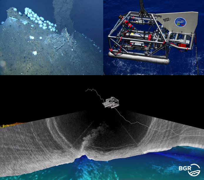
BGR conducts annual cruises into the contract area located along the Central and South-Eastern Indian Ridge. It has a size of 10,000 km², which is about the size of the island of Cyprus or Hawaii and is organized in 12 clusters consisting of 5 to 17 blocks of 10 × 10 km² each. To detect new hydrothermal vent sites, at first, likely areas for hydrothermal activity are identified using ship-borne bathymetry. Then, a “plume-hunting” sled equipped with chemical sensors for temperature, oxidation-reduction potential, and turbidity, is deployed to detect water column anomalies. If such water column anomalies have been detected, the BGR-developed deep-towed MBES sled HOMESIDE (Fig. 1 top right) is deployed in the area of potential origin of the anomaly. It is towed about 100 m to 120 m above the seafloor in 3,000 m water depth, allowing to obtain terrain models of a resolution of 2 m. This is sufficient to map the sulphide mounds in adequate detail. But more importantly, in regard of localization of the discharge site, the hydrothermal plume can directly be visualized within the MBES water column data. In Fig. 1 bottom, a 3D visualization of the bathymetry, HOMESIDE and real swath water column data collected over a venting site are shown. The HOMESIDE data is streamed in real-time during acquisition to the lab via the towing cable. Therefore, the acquisition parameters can directly be adjusted accordingly. Unlike active venting, inactive sites do not discharge hydrothermal fluid and therefore no water column anomaly can be used for their detection. Therefore, since 2019, a string for the detection of self-potential anomalies has been added to HOMESIDE. A self-potential anomaly is an electric field that forms in the seawater over a metal-bearing area in or on top of the seabed. To detect it, the voltage between different electrodes is measured in an array attached at the lower end of the string. Such anomalies can indicate sulphide deposits whether a site is active or not. To allow the probe to be as close as possible to the seafloor, the length of the string is about 90 m. After a new hydrothermal site has been located, camera carrying devices like ROVs or video sleds are deployed to gather visual information. It is also sampled to proof the occurrence of sulphides at the new site.

A high position accuracy of HOMESIDE data is crucial to correctly locate the hydrothermal sites, but also to reduce mismatches between overlapping bathymetric data. Due to sensor malfunction or operational errors, the navigation solution might not fulfil the high accuracy requirements. As a result, position mismatches of ROV deployments and bathymetric maps might occur. Furthermore, the mismatches in the overlap might reduce the visibility of small bathymetric features. This then decreases the ability to correctly identify potential interesting structures in DTMs, like inactive sites. Therefore, the bathymetric data needs to be further post-processed in case the navigation data exceeds an accuracy of about 10 m. In the following chapter the instrumentation and the data-based navigation correction are described.

3 HOMESIDE: Instrumentation and navigation correction in post-processing

The deep-towed sled HOMESIDE is equipped with a Kongsberg EM 2040 multibeam echo sounder. It is generally operated with 300 kHz (frequency modulated signal) and 400 soundings per ping when towed at an altitude of 100 m to 120 m. It is a dualreceiver MBES achieving typically a swath width of about 500 m. For navigation, the INS (Exail Phins 6000) is aided by an USBL (ultra-short baseline) underwater positioning system, a DVL (Doppler velocity log) Teledyne RDI Workhorse Navigator 600, and a CTD Valeport Midas SVX. Additional chemical sensors, like for turbidity and oxidation-reduction potential are also integrated on HOMESIDE for plume detection of active vent sites.

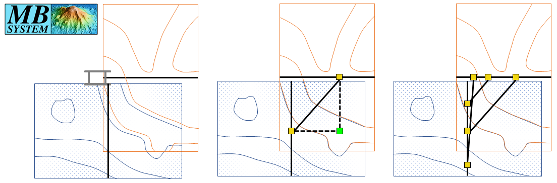
The utilized USBL system varies with the research vessel employed, therefore, over the years, multiple USBL systems have been used. BGR also deploys a mobile Sonardyne Ranger 2 USBL system and has used it additionally to – or instead – of the ship-owned system. The accuracy of the final HOMESIDE navigation depends largely on the accuracy of the USBL, which again depends mainly on the geometry (distance of transceiver and transponder) and utilized sound speed profile (SSP), assuming the calibration is valid. The accuracy of the HOMESIDE’s INS is given by the manufacturers as three times better than the USBL accuracy (Exail, 2018), which is about 0.2 % of the slant range for the Sonardyne Ranger 2 (Sonardyne, 2014). The distance between the vessel and HOMESIDE varies during one tow. It is typically shorter – and about the water depth – in the beginning of a deployment, and increases during the deployment as the ship speed is usually higher than the one of HOMESIDE. To maintain the altitude, the cable length has to be increased. If the distance gets too large, the communication of the USBL transceiver and the transponder can start failing occasionally. In such cases, the ship speed is reduced to improve the reception. With a typical slant range of 5,000 m, the expected positioning accuracy of the USBL is about 10 m and of the INS hence about 3 m (assuming no large systematic offsets due to drop outs of important aiding sensors for example). The real-time INS data is firstly post-processed by using the software Exail Delph INS. It allows a re-computation of the navigation by excluding certain aiding sensors (also just temporarily) or including additional ones, if they have been recorded separately. Further, smoothing filters can be applied. This way, the navigation can be much improved. But it does not include any corrections for incorrect SSP (e.g., in case an older one is applied). Due to time constraints, an SSP cannot be taken before each HOMESIDE tow, sometimes not even before the first station when starting the instrument deployment in a new cluster. Therefore, a slight decrease in accuracy can be assumed for stations where the SSP is older. The resulting effects are noticeable in the bathymetric data of HOMESIDE: Typically, mismatches between two adjacent data sets of up to 10 m can be expected. This is considered as no large systematic offset. If there are offsets of up to 50 m or so (e.g., due to completely wrong SSP or false calibration values), typically a dependency of the tow direction can be noticed. Such large offsets need to be adjusted, but minor mismatches reduce the quality of the final DTM and the ability to identify small bathymetric features as well.To reduce mismatches between overlapping HOMESIDE data sets in post-processing, the open source software MB-System is used. It is a software to process and visualize MBES and side scan data and was developed by the Lamount-Doherty Earth Observatory of Columbia University and is now maintained by the Monterey Bay Aquarium Research Institute (MBARI), University of New Hampshire, and MARUM. MB-System is LINUX-based and consists of numerous tools that can be executed within a terminal window. The main component used for the navigation adjustment is mbnavadjust. This tool allows relative navigation adjustment of data files based on features present in overlapping areas. In Fig. 2, the principle of the navigation adjustment in mbnavadjust is schematically depicted: Two overlapping files (represented in red and blue) show mismatches when comparing their bathymetry – represented via contour lines (left). For a certain location in the overlap (bright green square), the relative offset between the data sets is determined. The offset is stored as tie point in conjunction with the two corresponding navigation control points (yellow squares, centre). For each overlap, multiple tie points are set for different locations of an overlap, if possible (right). The tool offers an automatic determination of the offsets (in xyz or xy only), but also the operator can manually shift the data sets until they match visually and choose the shifting values as offsets to be stored. The tie points are set manually. When processing HOMESIDE data, typically, all data overlaps larger than 10 % are inspected and tie points are set.

After all tie points are set, a least square adjustment is performed, which tries to find the optimum fit of all data sets to each other by minimizing the offsets. The user has the possibility, to assign different weights to individual surveys: fixed (no adjustment), good (takes part in the adjustment), or poor (will be fitted after adjustment). The set tie points and the applied shifts can be inspected and changed if necessary. In Fig. 3, an example of a smaller data set is depicted. This data set has the advantage that, in the northern part, multiple data sets of different years were run over another, resulting in large data overlaps. On the lefthand side in Fig. 3, the DTM and the tie points are shown as connections between the navigation control points are shown (in cyan for ties within a survey and in blue for ties between different surveys). The right-hand side shows a model plot with the offsets after adjustment and which will be applied for longitude, latitude, and depth (top to bottom).

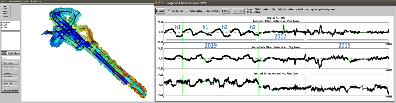
In the model plot, the different years of data acquisition are highlighted: 2015, 2017, and 2019. In 2019, the dual-receiver configuration of the MBES on HOMESIDE was used the first time. Both sensor heads were imported separately into MB-System, indicated by “h1” and “h2” in the model plot. Examining the offsets closer, large systematic offsets in the 2019 data of up to 50 m can be noticed (especially in longitudinal direction). Each of the four data sets of 2019, consists of two profiles run in opposite direction and the dependency on towing direction as well as cable length can be recognized: firstly, the offsets are small in the beginning, turns, and end of the station where the cable length is short. And secondly, the offsets have different signs (+/-) depending on the towing direction. These large offsets in this example occurred because an SSP of another area was applied in the USBL.

After navigation adjustment in MB-System, the new navigation is then applied to the original bathymetric data in the MBES bathymetry processing software QPS Qimera and finally edited. Within the editing process, wrong depth measurements are removed and small remaining mismatches in overlapping data reduced by excluding certain soundings from the DTM computation.

4 Results and discussion

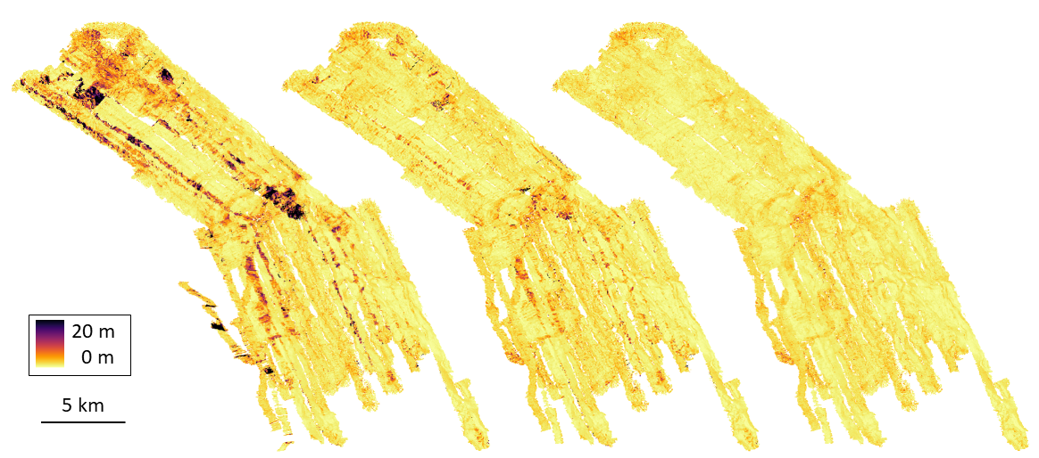
The best way to visualize the improvement of data quality, is the depiction of DTMs created from various data stages coloured by uncertainty (95 % confidence interval). The colours indicate therefore how good the soundings within one DTM cell (2 m) fit together. In Fig. 4, a large compilation of different HOMESIDE data sets collected between 2015 and 2022 is shown in different processing stages. The depictions are coloured by uncertainty: darker areas represent DTM cells where the sounding depths deviate stronger from each other than in the brighter cells. The data compilation consists of over 3,200 data files and 24,200 tie points were set manually. The improvement of how the measurements fit together is clearly visible from the left side (before MB-System) to the centre (after MB-System) and to the right (after final data editing).

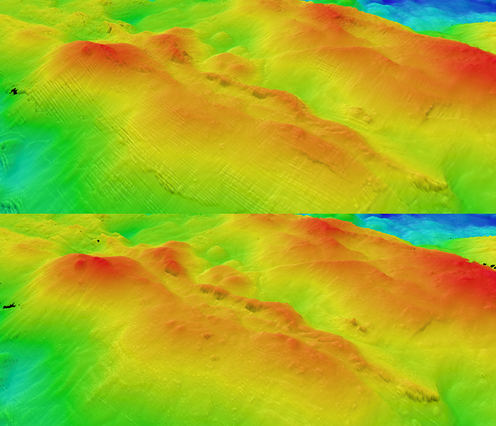
A section of the same data is shown in Fig. 5 in a 3D representation. The depiction on the top shows the data before and at the bottom after the navigation adjustment in MB-System. The artefacts caused by the navigation offsets can clearly be noticed in the top picture. Small mounds and other details in the bathymetry can be more clearly recognized in the bottom picture.

The disadvantage of using MB-System is the amount of manual work. It is very time consuming to set every tie point manually. For an intermediate sized data set, it takes about two weeks to set all tie points. The time can be reduced when decreasing the amount of tie points, but this influences also the quality of the adjustment. Furthermore, MB-System has the disadvantage that both MBES heads can only be imported separately. After the least squares adjustment, the two individual navigation solutions for each head are again averaged to one final navigation solution, which impairs the original results from the adjustment. Additionally, possible alternative tools to shift new data sets based on mismatches in the overlap to older data in a more time efficient way are tested.

5 Conclusion

Hydrothermal sites and the associated sulphide deposits are of interest as possible mineral recourses in the future. Research methods to explore and understand them are continuously improving. Hydrography plays an important role herein, as based on the MBES water column data discharge sites of hydrothermal fluid can be located. Furthermore, the bathymetric data allows the visualization of the investigation area, which in turn is the basis for further investigations and analysis. The data collected within this project is unique, as it is rare that such a large amount of data is collected over so many years in such a remote area and with such high requirements for accuracy and resolution. Whereas high accuracy positioning on the water surface is available, high accuracy under water positioning is still challenging and not easily achievable. The availability of MBES post-processing tools that provide possibilities for data-based navigation adjustment, is crucial for fulfilling the high data requirements for an underwater platform like in this project.

References

Baker, E. T., Resing, J. A., Haymon, R. M., Tunnicliffe, V., Lavelle, J. W., Martinez, F., Ferrini, V., Walker, S. L. and Nakamura, K. (2016). How many vent fields? New estimates on vent field populations on ocean ridges from precise mapping of hydrothermal discharge locations. Earth and Planetary Science Letters, 449, pp. 186–196. https://doi.org/10.1016/j.epsl.2016.05.031

Beaulieu, S. E. and Szafranski, K. (2020). InterRidge Global Database of Active Submarine Hydrothermal Vent Fields Version 3.4. PANGAEA – Data Publisher for Earth & Environmental science. https://doi.org/10.1594/PANGAEA.917894

Boschen, R. E., Rowden, A. A., Clark, M. R. and Gardner, J. (2013). Mining the deep-sea seafloor massive sulphides: A review of the deposits, their benthic communities, impacts from mining, regulatory frameworks and management strategies. Ocean & Coastal Management, 84, pp. 54–67. https://doi.org/10.1016/j.ocecoaman.2013.07.005

Exail (2018): PHINS 6000 Datasheet. https://rts.as/wp-content/uploads/2018/09/iXBlue-PHINS-6000-Subsea.pdf (accessed 1 October 2023).

Hannington, M. D., de Ronde, C. E. J. and Petersen, S. (2005). Sea-floor tectonics and submarine hydrothermal systems. In J. W. Hefenquist, J. F. H. Thompson, R. J. Goldfarb and J. P. Richards (Eds.), Economic Geology. Society of Economic Geologists, Littleton, Colorado. https://doi.org/10.5371/AV100.06

Hannington, M., Jamieson, J., Monecke, T., Petersen, S. and Beaulieu, S. (2011). The abundance of seafloor massive sulphide deposits. Geology, 39(12), pp. 1155–1158. https://doi.org/10.1130/G32468.1

Sonardyne (2014). Datasheet Sonardyne Ranger 2 USBL. https://www.uniquegroup.com/wp-content/uploads/2022/10/Sonar-dyne-Ranger-2-USBL.pdf (accessed 1 October 2023).

SPC – Secretariat of the Pacific Community (2013). Deep sea minerals: Sea-floor massive sulphides, a physical, biological, environmental, and technical review (E. Backer and Y. Beaudoin, Eds.), Vol 1A.