1 Introduction

The automation of geospatial data acquisition, processing and analysis is a widely researched field that is constantly advancing in terrestrial (Kraus, 1997; Longley et al., 2005; Van Genderen, 2011) and marine environments (Lurton, X, 2002; Jong, 2002; Wu et al., 2021). Optical measurement techniques such as LiDAR (Light Detection and Ranging) and underwater technology such as sonar (Sound Navigation and Ranging) allow large areas of land and water bottom topography and backscatter to be surveyed, producing highly accurate data that can be displayed as either 3D point clouds (Liu et al., 2021) or raster data (Schimel et al., 2018).

Seabed topography, morphology and subsurface characteristics are typically surveyed using hydroacoustic sensors such as side-scan sonar (SSS) and multibeam echosounders (MBES). SSS and MBES are suitable for comprehensive surveys of larger areas in deeper waters. Both sensor technologies provide backscatter information while MBES can also measure depth. The amount of data collected can be classified as Big Data, as a single survey can reach hundreds of millions of data points. Therefore, it is not feasible to perform analysis manually and data handling requires powerful computing and extensive storage solutions (Wlodarczyk-Sielicka & Blaszczak-Bak, 2020).

The need for widespread, accurate and up-to-date information on the shape of the seabed is critical for many marine economic and environmental purposes (Jonas, 2023). In particular, the identification of natural (e.g. boulders) and man-made subsurface objects is becoming increasingly important (Papenmeier et al., 2020). Boulders in particular pose a potential hazard to shipping. Their exact positions must be taken into account in nautical charts, especially in areas where minimum underkeel clearance is required (Mills, 1998). Boulders also provide habitats for many marine species and need to be considered when building or extending offshore infrastructure (Irving, 2009; Grzelak & Kuklinski, 2010; Wenau et al., 2020). Identifying objects such as boulders is also important for creating accurate Digital Terrain Models (DTM) by optimising established Computer Vision (CV) methods that separate ground points from the Digital Surface Model (DSM) generated by sonar and LiDAR (Förstner & Wrobel, 2016; Silva al., 2018).

Identifying small objects such as boulders in large datasets can be challenging. Current best practice, as outlined in official guidelines (Heinicke et al., 2021), recommends the manual identification of boulders when analysing large areas. This is achieved by processing the sonar data into a mosaic with a resolution of 25 cm per pixel and then manually interpreting the data. A grid with a resolution of 25 m × 25 m (coastal waters), 50 m × 50 m (Baltic Sea) or 100 m × 100 m (North Sea) is created for this purpose and categorised according to the number of boulders into three categories: no boulders, 1–5 boulders, more than 5 boulders. This workflow is inefficient, often taking several weeks to complete for larger survey areas, and is less suitable for producing DTMs.

Within the past decade, deep learning based computer vision has emerged for sonar data (Steiniger et al., 2022) and automated boulder detection from hydroacoustic data has been an area of interest for a number of researchers. Michaelis et al. (2019) trained a Haar-like feature detector on 300 kHz SSS data for a 12 km² study area within the Sylt Outer Reef, North Sea and could detect up to 62 % of the overall occurrence of boulders. Feldens et al. (2019, 2021) used the YOLOv4 model for object detection on both MBES and SSS data from the west of Fehmarn,

Baltic Sea. The highest mean average precision (mAP50) was 64 % for MBES (slope rasters), and 37 % to 43 % for two different detection models for SSS data. Feldens (2020) used deep learning super-resolution to address the limited resolution of many available side-scan sonar datasets.

Van Unen & Lekkerkerk (2021) demonstrated a classification model on a point cloud derived from MBES measurements, where each point is labelled as either boulder or seabed. The evaluation showed an accuracy of 35.5 %, with almost twice as many false positives as true positives for the boulder labels. The authors concluded that the algorithm is far from trustworthy, but can help surveyors with preliminary detections. Problems included a lack of data quality and quantity, boulders being only partially classified as such, and many small pebbles being detected that would not be classified as boulders. Similar issues arise in other areas of remote sensing, such as optical sensors: Bickel et al. (2019) detected lunar rockfall based on NASA’s Lunar Reconnaissance Orbiter narrow angle camera (NAC) images with an AP of 69 % for an Intersection of Union (IoU) of 50 %. Similar to the analysis of SSS data based on backscatter intensities, the analysis of the NAC images based on albedo is limited by a coarse spatial resolution of 0.5 m / pixel, and boulders are identified by an elevated albedo on their surfaces and a long shadow on the sides of the boulders.

Previously published approaches to boulder detection are based on academic case studies. In order to improve boulder detection for practical hydrography and habitat mapping requirements, existing approaches need to be refined and extended. Different hydroacoustic sensors and sensor settings need to be considered for a wide range of applications. It is also important to make these capabilities accessible to a wide range of hydrographic professionals. For this reason, it is necessary to make workflows easy to use. This can be achieved with a graphical user interface (GUI) and automated data processing routines that eliminate the need for coding or manual data transformation.

This study proposes a workflow that automatically detects boulders on both SSS and MBES data. It integrates with the existing data acquisition, processing and interpretation workflows of hydrographic and marine environmental professionals. Object detection algorithms based on Convolutional Neural Networks (CNN) are at the core of the application, but workflows including data management, pre- and post-processing are equally important, as most available AI tools and libraries are not specifically designed to work with hydrographic or geospatial data. A desktop-based user interface is presented to assist users with all key tasks, and a modular design allows for flexible expansion (e.g. support for new models and data types) in the future.

This paper is structured as follows: Section 2 outlines the methodology for AI-based boulder detection, detailing the tasks to be automated for different data inputs and different automated data workflows, as well as the configuration, training and evaluation of different deep learning models. Section 3 describes the software architecture and GUI. Section 4 presents the application of four different models to two different datasets collected using MBES and SSS sensors. The results are discussed in Section 5.

2 Workflows for automated boulder detection

2.1 Object detection of marine boulders

CNN-based object detection models were used to identify boulders in hydroacoustic datasets. A hydroacoustic dataset can be represented as a raster or a point cloud. In a raster representation, geographic space is divided into an array of rectangular or square cells to which attributes are assigned. These cells are sometimes referred to as pixels and form the elements of pictures, images or mosaics (Longley et al., 2005). The term grid, as used in the following, does not refer to the data representation or raster data, but to a network of equally spaced horizontal or vertical lines (Merriam-Webster, 2024), which may also delineate grid cells. 3D point clouds consist of a large number of 3D points. Each point consists of three coordinates that uniquely identify its location and optional attributes (Liu et al., 2021). This format is preferred for many applications related to scene understanding, as it preserves the original geometric information without any discretisation (Guo et al., 2019). Apart from the acoustic waveform, which is not analysed in this paper (Kubicek et al., 2020), backscatter intensities and bathymetry are the most common types of information included in hydroacoustic datasets. Fig. 1 shows how boulders can be visualised using this information and how they are annotated by experts as a basis for object detection. While MBES data include backscatter and bathymetry and can be represented as both point clouds and raster data, SSS data are mostly represented as raster data as they do not include bathymetry. The following Sections 2.3 and 2.4 describe workflows for each of these types of data representation separately, as they require different sets of tools and data preparation. However, several generic concepts form the common basis of both workflows and are explained in the following paragraphs and in Section 2.2.

CNN models for object detection tasks are typically trained on 2D or 3D data supplemented by annotations consisting of bounding boxes. Bounding boxes describe an approximate area in which an object is located by a surrounding rectangle in 2D space or a cuboid in 3D space. Trained detectors can predict similar bounding boxes with confidence scores between 0 and 1 for input data containing similar objects (Szeliski, 2022). Based on these conditions, we have identified the following set of basic tasks (T1–T6) that need to be performed: Boulders need to be annotated on hydroacoustic data (T1). Based on the hydrocoustic data and the annotations, a socalled ground truth (GT) dataset has to be created in the specific data format (T2) that is required for the training and validation of a specific CNN model (T3). A trained and validated model needs to be tested (T4) before it can be used to detect boulders on hydroacoustic data in a production environment (T5). The output of the detection can be post-processed to mitigate possible shortcomings of the output or to address specific user needs (T6).

Since experts have to create initial GT annotations manually, the annotation process has to be designed to meet their specific needs and habits of working with data (Fig. 2). Sonar datasets are usually visualised as large raster mosaics within a domain-specific application or a general-purpose GIS such as QGIS and ArcGIS. Within the large mosaics, Regions of Interest (ROI) are defined by polygons where annotations are to be created and later extracted from the original data. As boulders need to be distinguished from seabed and other objects, ROIs without boulders (here called empty ROI) are defined to collect examples of the latter features (similar to Feldens et al., 2021). Allowing experts to define ROIs within a larger dataset is also a means of creating a balanced dataset with sufficient variability.

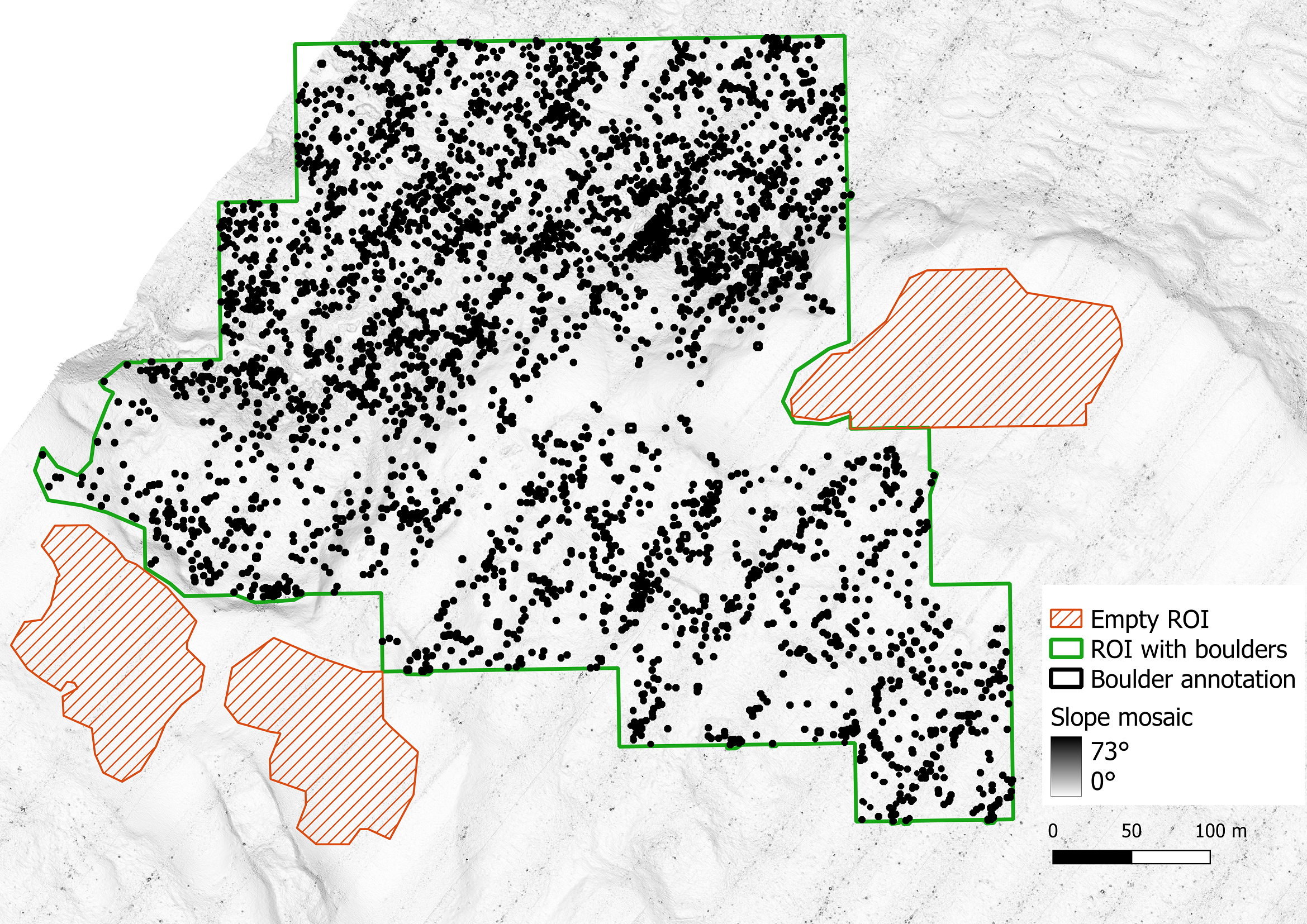
CNN used for image analysis cannot process large continuous datasets as a whole. Instances of input data are limited to a few thousand pixels or data points, depending on available memory. Therefore, for both raster and point cloud analysis, the data must be retiled or sliced in order to be processed iteratively. This approach is similar to that reported by Feldens et al. (2021) and Bickle et al. (2019). Thus, all input data are overlaid with a regular grid, where the cell size and the overlap between the cells are defined depending on data resolution, object sizes and model characteristics (Fig. 3). It is necessary to define the overlaps because some objects are only partially included at the grid cell boundaries and are therefore difficult to detect. An overlap larger than the size of the expected objects ensures that all available data from each object are included in one grid cell. Cases where objects occur in more than one grid cell due to the overlap, or where objects are truncated at the cell boundaries, must be dealt with by deduplication at a later stage in the workflow. The size of the data slices is limited by the hardware used, such as the performance and memory of the graphics card, and the way in which the chosen algorithm uses it. Working with larger slices results in fewer overlapping areas to deal with, but may result in larger areas of no data at the boundaries of an ROI.

A common pattern for training and evaluating models in machine learning and deep learning is to split the GT data into three parts: A large training dataset for iteratively optimising the model weights and hyperparameters during training, a smaller validation dataset for monitoring error (or performance) metrics during training and selecting the best weights (early stopping), and a test dataset for evaluating the model based on data not involved in training (Lakshmanan et al., 2022). The division between training and validation data in this paper is done by randomly assigning data slices to either the former or the latter in a ratio of 9:1. This ratio is maintained for each ROI as well as for the input dataset as a whole. Since the number of data slices within an ROI is not always divisible by 10, the absolute counts of the assigned slices are rounded to the nearest integers. The test dataset in this work is completely separated from the training and validation data.

For many CV and machine learning tasks, extensive reference datasets exist for benchmarking and comparing algorithms, such as ImageNet (Deng et al., 2009), MS COCO (Lin et al., 2014) and Pascal VOC (Everingham et al., 2014) for image-based tasks and the KITTI (Geiger et al., 2013) and Waymo (Sun et al., 2019) datasets for tasks on 3D objects, point clouds and autonomous driving data. The most common metrics for evaluating such object detection tasks in both 2D and 3D spaces are the mean Average Precision (mAP), an average of all Average Precision (AP) values across different classes or categories, and the Intersection over Union (IoU; Hosang et al., 2016). As the datasets in this paper contain only one class and category, namely boulder, the distinction between AP and mAP is not made. However, the mAP is a primary measure for evaluating object detection as it combines multiple important metrics and model outputs into one value. The IoU is based on pairwise comparisons of GT bounding boxes with predicted model bounding boxes, where the common intersection area is divided by the combined area of both shapes, i.e. two identical boxes have an IoU of 1 % or 100 %.

An IoU threshold determines the AP and the measured number of true positives TP (predictions that match a GT box), false positives FP (predictions that do not match) and false negatives FN (GT boxes with no matching prediction), which the metrics precision TP/(TP+FP) and recall TP/(TP+FN) are calculated. In practice, different IoU thresholds are used for AP calculation depending on the task, but it is common to use either a threshold of 50 % or to perform multiple calculations with different thresholds between 50 % and 95 % and calculate the average (Hosang et al., 2016). A high precision model will have few FPs relative to its TP, without any indication of how many GT instances were actually predicted. High recall indicates that many GT boxes are matched by predictions with no indication of FP. Ideally, a model should have both high recall and high precision. However, by filtering predictions with confidence threshold, the model’s output could be optimized for either precision or recall. The AP combines precision and recall by calculating an average over different confidence thresholds (e.g. over the precision/recall curve). All of these metrics are also used, with some variation, by the AI libraries and tools described in this paper. They can be given either as values between 0 and 1 or as percentages. As a convention in this work, all mAP, IoU and recall values are expressed as percentages. IoU thresholds are indicated by a number appended to the metric, e.g. mAP-50 for a threshold of 50 %.

2.2 Technical challenges

Most of the available AI tools and libraries, in particular those used in this work (Darknet, MMDetection3D and the Ultralytics framework), are not designed for processing hydrographic or geospatial data. This poses several challenges: If the work is based on such tools, the input data have to be converted into other data formats with a possible loss of information, i.e. the coordinate reference system, among others. For the output, in turn, spatial references have to be derived from the context of the input. Information on how to transform hydrographic information into non-hydrographic formats and how to contextualise non-hydrographic output with domain knowledge needs to be maintained separately.

It is not only the object detection algorithms that are not ideal for large geospatial and hydrographic datasets, but also the established annotation tools, such as Label Studio¹ for image data and CVAT² for image, video and point cloud annotations. In the context of this work, many of the available and framework-compatible tools for 2D image annotation are designed to annotate images of normal image size rather than larger mosaics. The tools available for point cloud annotation are also designed to annotate smaller 3D scenes and do not perform well on multi-gigabyte (GB) datasets. Although it would be possible to first slice the sonar data and then annotate each tile using one of these tools, there are several drawbacks to this approach: Annotations are created in image coordinates or local 3D coordinates and stored in a specific format compatible with a family of algorithms (e.g. YOLO or KITTI format). Geospatial references are not retained, making it difficult to contextualise or integrate these annotations with other hydrographic or geographic information. It would be more difficult for experts to select ROI or get an overview when working from scene to scene than when working with the whole dataset, and they would have to learn to work with new software. It was therefore decided instead, to use established GIS software to draw geographically referenced polygons around boulders, and to write data converters to transform this data into specific annotation formats (Feldens et al., 2021). This approach is also more versatile, as it allows the same data to be reused for different algorithms and grid schemes, depending on changing hardware and software requirements.

The hardware and software requirements also specify the selected AI tools and settings. The experiments and software development were mainly carried out on a Windows 10 workstation computer with an NVIDIA 3080 Ti graphics card. The aim of this work is to enable boulder detection on similarly equipped desktop or server computers. Key considerations for the software and algorithms used in this work include the availability as an actively maintained open source implementation, sufficient stability, and applicability to common object detection use cases.

2.3 Raster-based boulder detection

A previous study by Feldens et al. (2021) used YOLOv4 (Bochkovskiy et al., 2014), implemented on the open source framework Darknet³ as a backbone for raster-based boulder detection. The current work reuses parts of the publicly available source code⁴ and workflows and partially incorporates the newer model architecture YOLOv8⁵, based on PyTorch.

The hydroacoustic data input to this workflow is expected as pre-processed raster files in GeoTIFF format, i.e. gridded sonar data with a resolution of 25 cm × 25 cm per pixel. Data pre-processing is specific to the input types, and is described, for example, in Wilken et al. (2016) for SSS imagery, in Lurton et al. (2015) for MBES backscatter imagery and in Gao (2009) and Ferreira et al. (2022) for bathymetric datasets. Feldens et al. (2021) explored different types of raster derivatives and how well they perform for boulder detection. Based on these publications, it was decided to train SSS-based models with backscatter rasters and to train MBES-based models on rasters of slope values calculated from bathymetry rasters (QGIS.org, 2024). Experiments with YOLO4 and bathymetry rasters, and composite images combining bathymetry resp. slope with backscatter data into multi-channel images, confirmed previous findings that they give worse results than slope data alone (Feldens et al., 2021). These examinations are therefore not included in this paper. Slope data is preferred to hillshading because the latter conversion is more deterministic, results in a fixed range of values between 0 and 90 degrees, and eliminates the absolute depth as a variable from which boulder detections should be independent. The YOLOv4 implementation used is only compatible with 8-bit greyscale images and 32-bit RGB images, which means that each raster cell in a band can only have an integer value in the range [0,255]. Whilst absolute depth values would be constrained by this limitation, slope values could still be represented with reasonable accuracy above the sensor accuracy. The GeoPackage (GPKG) was chosen as the file format for both vector input (boulder annotations and ROI) and detection output.

The first automated step in the raster-based workflow, after data pre-processing and GIS-based annotation (T1), is the creation of a training dataset (T2), as shown in Figs. 4 and 5, divided for visual purposes only. Larger segments of the input raster files are extracted by overlaying them with the polygons defining ROIs (Fig. 4). Rotated copies of these slices are created at different angles, so the CNN is trained with the data of different orientations and learns to recognize boulders independent from their alignment. Rotating larger mosaics instead of small tiles also has the advantage that rotations that are not multiples of 90° will later result in tiles without edges that have no data. Therefore, it is not necessary to crop and scale these tiles to remove the edges. Next, the slices are divided into small, slightly overlapping tiles of the same size and scale, small enough to be more effectively processed by the CNN.

Once these tiles have been created, it is then determined for each tile whether and where there are boulders in the image (Fig. 5). Since GeoTIFF images can be processed like TIFF images without losing their spatial reference, the overlap between annotations and tiles can be determined using conventional spatial joins. For each tile, a text file is created with the image coordinates of all boulders. Bounding boxes that are partially visible within a tile are included if their dimensions equal or exceed a defined threshold of 75 cm in width and height of the height intersection area, which is equal to 3 pixels in width and height for the given resolution of the input data. In order to not exclude very small boulders by this threshold, bounding boxes are also included if they are at least 25 % visible in width and height. Partially visible bounding boxes are cropped to the visible area of the respective tile. These thresholds are based on empirical reviews of the data where artefacts of 2 pixels or less in either width or height could not be identified as boulders.

Finally, the tiles are randomly divided into training and validation datasets (Section 2.1). As it was found that a disproportionately large number of empty tiles leads to inefficient training with a very slow increasing mAP, it is also possible to limit the percentage of these tiles compared to the tiles with boulders. A limit of 40 % was used in this work.

Training and validation (T3) are entirely performed by the backend software (either Darknet or PyTorch, depending on the model used). The software is configured by the user, facilitated by a GUI. Tested default values are suggested by the software. Various data enhancement techniques such as mosaicking, rescaling, adding noise and varying saturation are also performed internally.

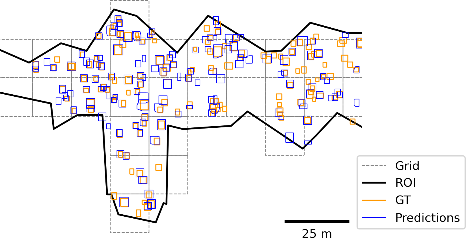
The test (T4) is carried out separately by comparing the GeoPackage of boulder annotations from the test dataset with the GeoPackage of detections, taking into account the defined ROIs. Python converters are written to extract the boundaries of each polygon and convert them to the bounding box format expected by the TorchMetrics Python package. The GT and detected data are then filtered and grouped by ROI. If the ROIs are irregular in size and shape, or if they contain much more than 100 GT annotations, it may be necessary to impose a regular grid on the ROI in order to efficiently calculate accurate performance metrics, as shown in Section 4.3.

Fig. 6 shows how the boulder detection (T5) and optional post-processing (T6) are implemented and automated. Similar to the GT data, the input data has to be retiled. The premise of this work is that optimal results are obtained when the tile size is the same as for the GT data, although empirical tests have shown that reasonably good results can be obtained with slight variations in tile size and with adjusted user-defined settings. The detection model predicts bounding boxes in image coordinates relative to the dimensions of each tile. Since GeoTIFF tiles contain geospatial metadata, these local coordinates could be transformed into the coordinate reference system of the input data. All georeferenced bounding boxes are then merged as polygons into a single GeoPackage file.

The model results in their current implementation often have the drawback of detecting the same boulders multiple times, due to the edge case of overlapping tiles (Section 2.1), but also due to properties of the predicted annotations and the algorithm itself. To eliminate these duplicates in a heuristic way, the clustering algorithm DBSCAN (Density-Based Spatial Clustering of Applications with Noise; Ester et al., 1996), as implemented by the Python package Scikit-learn⁶, can be applied, using user-defined weights as criteria. In summary, DBSCAN considers objects to be part of a cluster if they are reachable from each other according to a distance function that produces a numerical value that should be below a defined threshold.

This distance function has been replaced by a custom function that only considers overlapping bounding boxes and distinguishes between pairs of bounding boxes that originate from different tiles (edge cases) and those that have a high degree of overlap for other reasons, such as the shadow of a boulder, which is sometimes detected as a second object nearby. The likelihood that two bounding boxes are unique (not duplicates) is computed as a value between 0 and 1. In the first case, where bounding boxes originate from different tiles, the likelihood is computed from the minimum relative separation of two shapes, i.e. 0 indicates that one bounding box is completely contained by the other and 1 indicates that there is no overlap. In the second case, the likelihood is aggregated from three factors: the minimum relative separation, the relative similarity of the areas, and the similarity ratio of width to height. The threshold below which two bounding boxes are considered duplicates and the weighting of each factor in the likelihood calculation are determined empirically.

If a cluster is found, all polygons are merged into one entity using a convex hull. The maximum of all included confidence values is used as the merged cluster detection confidence. Since the worst case complexity of DBSCAN is O(n²), execution is accelerated by pre-clustering based on a safe threshold of Euclidean distance (larger than the largest observed object), taking advantage of the better performance of the built-in distance metric as opposed to the custom metric.

2.4 Point cloud-based boulder detection

The MMDetection3D⁷ platform for general 3D object detection (Zhang 2023) is used for the training, validation and boulder detection of MBES-based point clouds. The platform supports a variety of algorithms for point cloud-based object detection, although they have so far been developed, tested and applied to LiDAR data and not to sonar data. It is assumed that MBES-based and LiDAR-based point clouds are similar enough to apply these algorithms to the given use case. The specific algorithms used here are SECOND (Sparsely Embedded Convolutional Detection; Yan et al., 2018) and SAASSD (He et al., 2020). On KITTI test data with LiDAR point clouds, SECOND reached an AP-70 between 65.82 % (category hard) and 83.34 % (category easy) and SA-SSD reached 74.16 % (hard) and 88.75 % (easy) (He et al., 2020).

Due to the early stage of development, the point cloud-based workflow is not as sophisticated as the grid-based workflow described above. The partitioning of the data, the creation of the GT data and the recognition are inherited from the raster-based approach. The only difference is that instead of retiling raster files, files of 3D points are grouped and optionally split into training and validation data. Groups or sections of points are not explicitly rotated because MMDetection3D can be configured to perform rotations and other geometry manipulations internally. In the current version, GT data is initially annotated in the same way as the raster-based approach, i.e. by drawing 2D polygons in QGIS based on a mosaic file. A converter has been written that converts these polygons to 3D bounding boxes and estimates height / depth based on the shallowest and deepest points that fall within the area of the box. The results are checked and adjusted on a random basis.

The 3D geometries (Fig. 7) used to train the point cloud models are based on UTM projected geographic coordinates and depth. MBES backscatter is introduced as additional information. The MBES data are provided as comma-separated values (CSV) files, where each row represents a data point, including geographic coordinates, depth, signal intensity and beam angles. As part of the data pre-processing, experts have already flagged erroneous data in these files so that they can be excluded from the point cloud. The data points are not presented in any spatial order, but in the chronological order in which they were recorded by the MBES, with each file representing a track line followed by the survey vessel. As with the raster-based approach, the point cloud is usually much too large to be used directly as input data for model training. Instead, the point cloud needs to be broken down into smaller data slices that the AI backend can sequentially process with the available hardware (i.e. graphics cards). Intermediate processing steps using Python also require data slicing, as loading a dataset with millions of data points into the main memory exceeds the capabilities of many desktop and server computers.

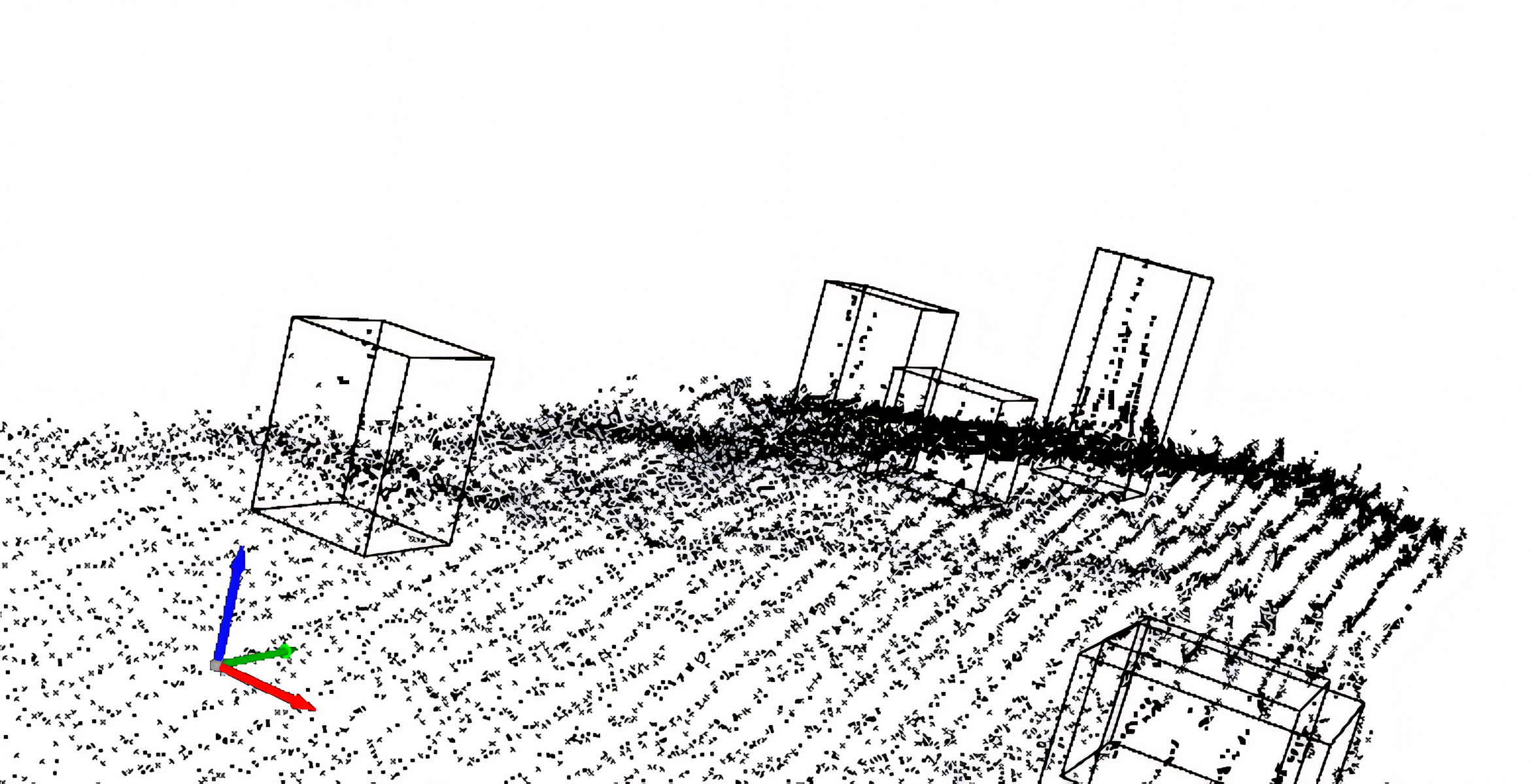
The chronological sorting of the points in the raw data does not allow direct partitioning into smaller spatially organised subsets. Due to the large number of points, it is necessary to reorganise and subdivide the data in an efficient and hardware-friendly way: First, all CSV files are read and appended to the same GeoPackage file. Since GeoPackage uses a SpatiaLite database internally, the data can then be queried according to a given spatial extent (bounding box of a grid cell). For the full extent of the dataset, which can also be queried, a spatial grid is constructed where each grid cell is defined by width, height and an overlap with neighbouring cells. Ground truth datasets are then constructed based on all grid cells that overlap with any region of interest. For each grid cell, all data points within the cell and an ROI are written to a separate file. All boulder annotations that overlap (at least partially) both the cell and the ROI are written to an associated annotation file. In this way, the boulders that are only partially visible within the cell are also annotated. The resulting dataset conforms to the standard layout of KITTI datasets (Geiger et al., 2013) and the requirements of the MMDetection3D software documentation for this type of data.

An optional pre-processing step is the de-trending of depth values, which is similar to ground filtering procedures (Silva et al. 2018; Gomes et al. 2023): For each 3D point, the mean depth of the k nearest neighbours is determined using the k-nearest-neighbours search algorithm of the library Open3D, based on FLANN (Muja et al., 2014; the experimental setups mentioned in Section 4.2 used k=200). The actual depth of the points is reduced by this mean depth. The resulting residuals are then used for training and validation data.

For the detection output, 3D bounding boxes are converted and merged into similar GeoPackage files as for the 2D raster-based approach (Section 2.3), but with the bottom depth and the height of each box included in their attributes. As a result, the same optional deduplication methods can be applied and detection performance can be evaluated in 2D space on the same test data that are used for the raster-based models.

3 Software design and realization

A software architecture and a prototype graphical user interface are presented below. They allow seamless integration into the operational workflows of potential users such as hydrographic offices and scientific institutions.

3.1 Software architecture

The software is written in Python 3.10 and was initially based on the public source code published by Feldens et al. (2021). It has been developed from a set of command-line processing tools to a modular software where data representation, workflow functionality and GUI are structured in packages. These types of modules form a functional division of the software into three layers, where the user interface (presentation layer) executes methods from the workflow modules (logical layer). Both the GUI modules and the workflows use object-oriented representations of the data layer for input and output. The data layer has no dependencies on workflows or the GUI, and the workflow has no dependencies on the GUI and can be used by itself as a Python interface. Darknet and MMDetection3D each serve as the AI backends of the software. Due to the modular design, other backends can be added as they become viable for boulder detection and similar tasks. The generic workflow package is the common (non-graphical) interface for all backends and provides Python methods for the tasks T2–T6 described in Section 2.1. GIS-based annotation (T1) is not implemented in this software.

The application uses the NumPy and pandas libraries for data processing and numerical operations. Several open source libraries are used for processing geographic vector and raster data, such as GeoPandas, PROJ, GDAL and OGR. The GUI is based on Tkinter (Python interface to Tcl/Tk) and is therefore designed for desktop use. As the software is modularised, different interfaces such as browser-based UIs can be added in the future. In order to organise the data in an efficient way, users can define local workspaces with respect to the workflow, so that input data, derived GT datasets, model configurations, trained models and detected data are organised in separate folders. This is useful because each of these data types can have a one-tomany or many-to-many relationship with the others, i.e. the same input data can be used to create a GT dataset, and a GT dataset can be composed of different input data. Similarly, a model configuration and a GT dataset can be reused to train different models. Models and data can also be shared separately for re-use by other users.

3.2 User interface

In order to make automated boulder detection accessible to non-programmers, a GUI has been developed (Fig. 8). The current version of this interface consists of four horizontal tabs, each corresponding to an automated workflow task (T2: training data preparation, T3: model training and validation, T5: detection, T6: post-processing). A testing interface (T4) will be added in the near future. Each tab contains an input form with mandatory file inputs and outputs and optional settings. All settings can be saved as JSON files, shared as such and reloaded on different machines. It is planned to develop this interface further in response to user feedback. Different interfaces will be possible in the future, such as a cloud-based server application programming interface (API) and a browser-based GUI.

4 Showcase Baltic Sea

4.1 Ground truth data

Fig. 9 shows where the GT data were collected in the German Baltic Sea. An MBES dataset M-TR from the Kadetrinne and an SSS dataset S-TR from the Western Rönnebank are used for training and validation of the boulder detection models. An MBES dataset M-TE and an SSS dataset S-TE were also acquired within the Western Rönnebank for testing purposes. For the S-TE test dataset there are two different subsets. S-TE1 was collected in 2022 and is based on a different survey than S-TR, which was collected in 2020. S-TE2 is based on the same survey as S-TR. The boulder annotations of M-TE, S-TE1, S-TE2 are based on approximately the same ROIs. None of these ROIs overlap with the ROIs of S-TR.

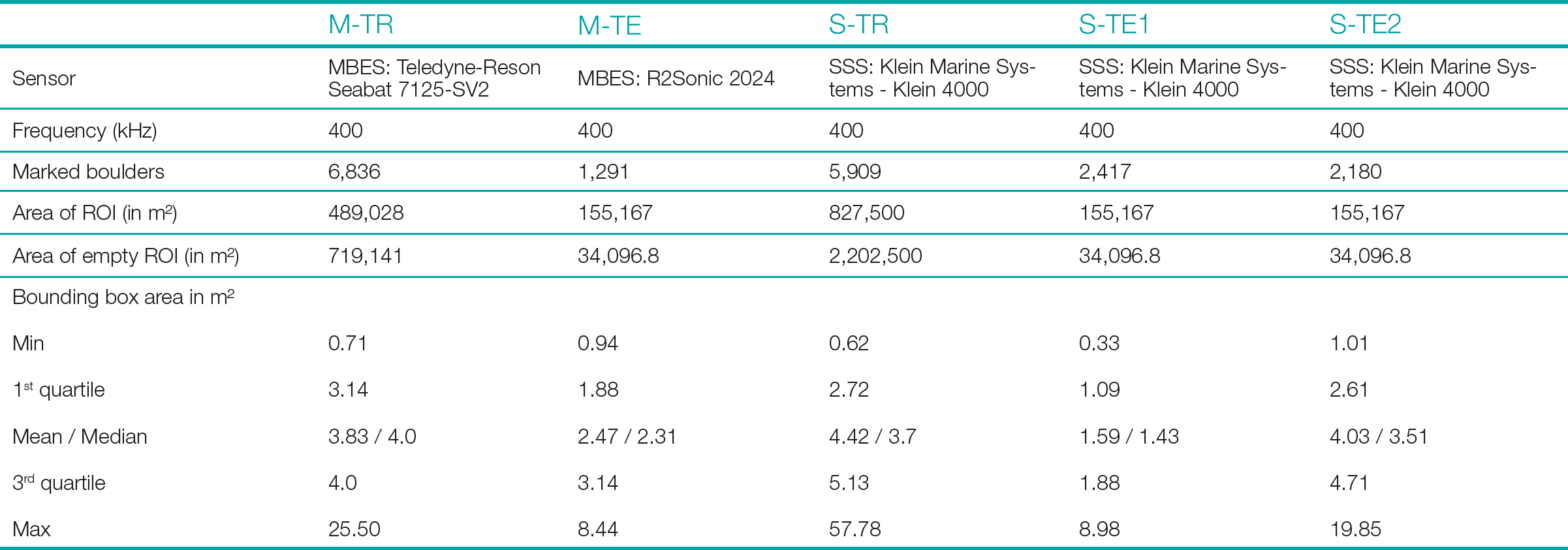
From the key statistics in Table 1, it can be seen that approximately 6,000–7,000 boulders were annotated for each training dataset and a few thousand boulders were marked for testing. All four datasets were annotated by the same expert by the method described in Section 2.1.

However, the sizes of the bounding boxes are not equally distributed between the training and test data. This is particularly obvious for the dataset S-TR and S-TE1 in comparison (Fig. 10). As all the raster mosaics were rasterized to a resolution of 25 cm × 25 cm per pixel, it can be estimated that the mean bounding box in the S-TR (the largest mean) covers about 71 pixels, while the mean for the S-TE1 is only 25 pixels. One reason is that for S-TE1, the sonar device was towed in a higher altitude by the vessel, with a difference in altitude of 2-4 m. That causes boulder shadows and boulders in general to appear smaller to humans. For S-TR and S-TE2, on the other hand, the distribution of bounding box sizes is similar because the tow altitude and detailed device settings are consistent across both datasets. Similar biases in the distribution of bounding box sizes could be observed for M-TR in comparison to M-TE, although the differences are smaller.

The datasets contain various gaps where data are missing due to measurement errors. Manual inspection showed that some boulders with data gaps could only be detected after filling these gaps by interpolation based on the neighbouring values. However, no significant changes in mAP and IoU could be observed for training with and without filling the gaps in the GT data, possibly because not enough instances of boulders with gaps were part of the validation data.

For M-TR and M-TE, the same annotations for boulders and ROIs were used for both point cloud-based and raster-based boulder detections.

4.2 Model training and validation

The models presented in this paper are the empirical results of 68 documented model training runs, where the training dataset as well as the hyperparameters were iteratively adjusted for optimal results, guided by the validation data. 16 experiments were performed on rasterised SSS data using YOLOv4, 13 on rasterised MBES data using YOLOv4 and 34 on point cloud-based detection using MMDetection3D. Five experiments were performed on YOLOv7 and YOLOv8 with promising results for YOLOv8 (Table 2). Many of these experiments failed due to poor neural network configuration, hardware and software limitations, or very low performance measurements for the validation data. A common reason for poor performance was an inappropriate ratio of network resolution to tile size, which was resolved by increasing the former or decreasing the latter. For MMDetection3D, mAP-50 values did not converge and did not exceed 15 % during trainings with object noise turned on, a setting that rotates and translates points only within 3D bounding boxes. After manual inspection of the boulder detection results, the training data was revised several times in order to ensure that many different views of boulders and the seabed are represented and accurately annotated. In cases where promising results were achieved, the hyperparameters of the neural network (i.e. resolution, learning rate) and the setup of the training dataset were iteratively optimised. For the rasterised MBES data, the best results were obtained with slope-converted data. Experiments with combined bathymetry and backscatter values (e.g. slope values in the R-channel and intensity values in the G-channel of an RGB image) performed worse than slope data alone, which is similar to the findings of Feldens et al. (2021).

Table 2 shows the main results of the study. For each model, the performance metrics (mAP and IoU) were reported by the libraries used (Darknet, MMdetection3D and Ultralytics). Using the above methodology, YOLOv4 achieved a mAP-50 of 65.66 % on SSS backscatter data. However, the result required a workaround for the often-reported weakness of YOLOv4 to not detect small objects well: The tile size was set to 60 px × 60 px, and although the network could be trained with a resolution of 608 px × 608 px on the given hardware, using larger tiles would lead to much worse results. However, model WRB-HF-8c was trained and validated using the exact same GT dataset as WRB-HF-8b, but with all tiles scaled up to 608 px × 608 px using cubic resampling. Although the average IoU is lower for the selected best weights, the mAP-50 increased by almost five percentage points. The same GT dataset was also used to train the YOLOv8 model, with a further improvement of over 8 percentage points. The advantages of YOLOv8 over YOLOv4 could not be further investigated at this stage. With a mAP-50 of around 70.46 %, MBES / slopebased boulder detection performs in the same range or slightly better than backscatter intensities on their respective validation data.

The trials of the point cloud-based models SECOND and SA-SSD achieved mAP-50 and recall-50 values of 24.15 % / 41.85 % and 44.02 % / 48.89 % respectively, based on 3D instead of 2D bounding boxes. An increased recall was measured for KDR-V34, i.e. many bounding boxes from the GT were recognised, albeit with a low accuracy of the IoU. However, the low mAP and visual inspection indicate that the model produces a high number of false positives with the given configuration. The SA-SSD-based model was trained on depth residuals rather than absolute depths. Although the mAP-25 and recall-25 are both lower than for KDR-V34, the results for mAP-50 and recall-50 are better, with fewer indications of false positives. However, the SA-SSD model could not be investigated further due to technical difficulties. Not shown in Table 2 is a model based on SECOND trained on depth residuals. This is because the results were very similar to KDR-V34 and were therefore considered redundant.

4.3 Model testing and comparison

This section describes how the trained models that performed best on their respective validation data (10 % of the tiles from M-TR and S-TR) were applied to the M-TE and S-TE test datasets and finally evaluated. Overall, all models perform worse than on the validation data. This is to be expected, as the datasets are not involved in the training, but also due to other differences such as the discrepancy in the bounding box size distribution.

Fig. 11 shows GT data and boulder detections for a small area of approximately 420 m². The small numbers in the boxes indicate the confidence of the prediction, ranging from 0 to 1. Predictions less than 0.1 have been suppressed for all models except KDRV34. For KDR-V34, the number of predictions with low confidence was so high that the filter had to be set to 0.15 in order to obtain a useful output based on visual assessment. From visual observation, the model with the best fit to the GT data is KDR-Slope-1d and the WRB-HFc model in respect to S-TE2 only. KDR-V34 makes plausible predictions for boulders that are easy to detect, but the false positives degrade the result. Both SSS-based models fail to predict small bounding boxes, particularly in S-TE1.

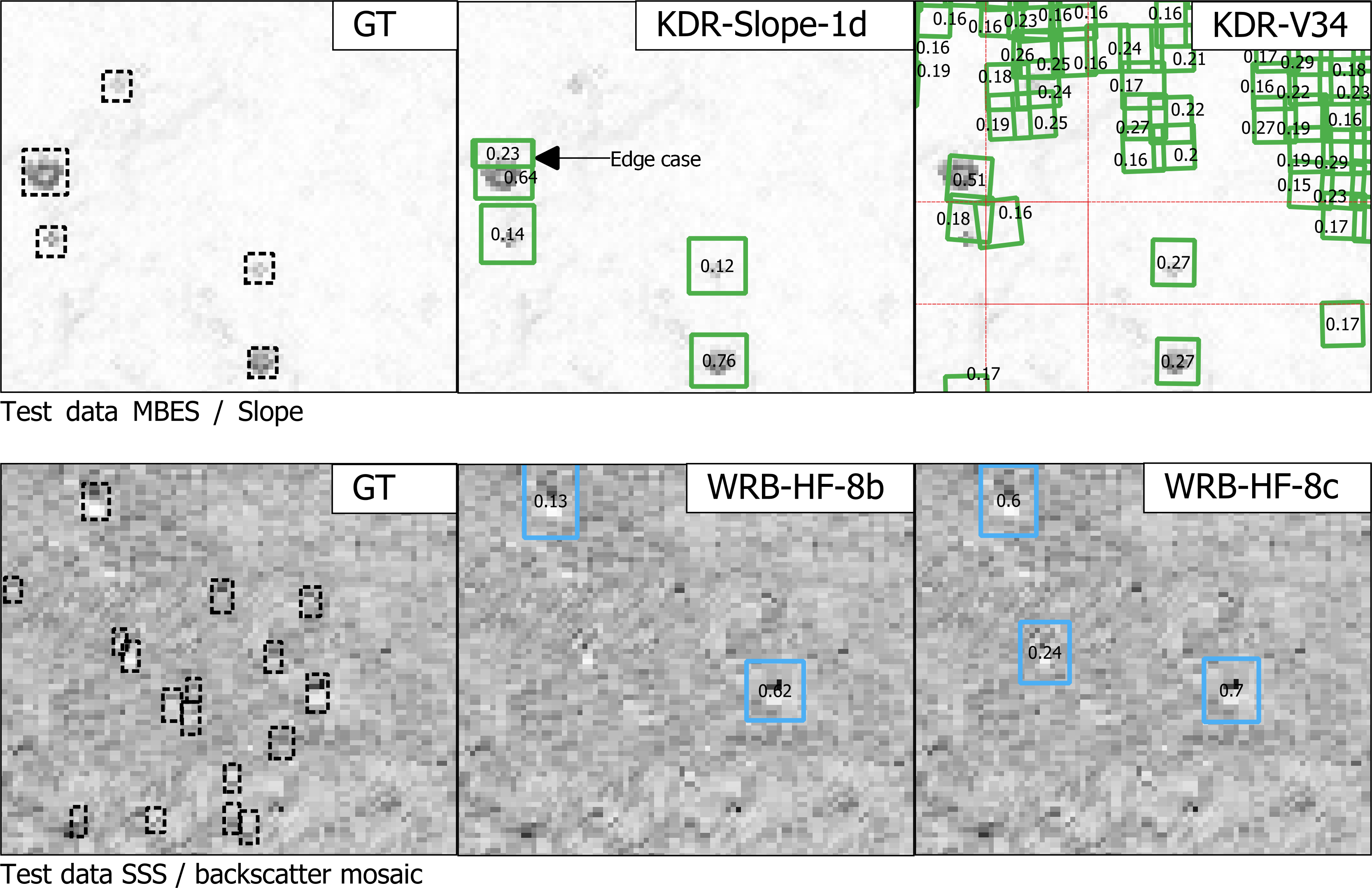
Table 3 and 4 show the performance metrics of four models and basic statistics of the GT data of the test regions. Each performance measure includes two values per model: the first value is derived from the output of the detection workflow, and the second from the deduplicated predictions. For each ROI, the predictions and GT annotations were used as input to the Python package TorchMetrics, using the package pycocotools as a backend to calculate metrics such as mAP and IoU. Pycocotools is based on the official API used to benchmark object detection and segmentation models (Hosang et al., 2016) on the MS COCO dataset (Lin et al., 2014), and is integrated into several applications, including YOLO8 / Ultralytics and MMdetection3D. Typically, object detection images are computed individually per image and then aggregated across all images and object categories. However, for evaluating boulder detection tasks, the area over which GT and predictions are compared is critical. Calculating metrics per ROI without considering the irregular areas of the ROIs, especially for M-TE and S-TE, would lead to biased aggregation results. The scoring algorithm also becomes inefficient if too many predictions are included per image. By default, the number of predictions evaluated is limited to 100. Therefore, it was decided to overlay a grid and thus compute and aggregate detection metrics for equally sized grid cells (Fig. 12). A bounding box is included in an input slice if at least 50 % of its area is within the corresponding grid cell. The cell size of 15 m × 15 m was empirically chosen to closely match the shapes of the grid and the ROIs and to keep the number of predictions per grid cell sufficiently low. At the same time, the number of grid cells should be small in order to avoid edge cases. Tables 3 and 4 show the detailed results of the test evaluation. The differences in the GT area and the number of GT instances compared to Table 2 are a result of the gridding process.

5 Discussion

Data acquisition in the marine domain is time consuming and therefore expensive, and the collected data must serve multiple purposes (“map once, use many times”). It is therefore necessary to have efficient data processing and analysis techniques at hand. As we show in this study, boulder detection is possible with high accuracy and reliability from different input data (data and data derivatives from MBES and SSS) supported by the developed workflow.

Some disadvantages of SSS-based boulder surveys are evident from the drastic decrease in mAP (Table 4), down to 0 for mAP-50, for SSS models, depending on the test area. The appearance of boulders in SSS data does not reflect their true geometry, but is a result of the insonification angle (similar to work on lunar rockfalls, Bickel et al. 2019). This depends on the distance of a boulder from the side-scan sonar and the tow geometry, and may contribute to a different appearance of boulders at a survey site compared to the training dataset. For site S–TE1 (Fig. 10) this resulted in apparently smaller boulders that the trained model was unable to detect. Where the boulder characteristics were similar between test and training sites (site S–TE2, Fig. 10 and Table 4), the results of the model trained on SSS data were in line with the expected performance based on the validation datasets. The MBES data more closely represent the actual boulder geometry and are therefore less affected by changing survey geometries (the resolution still changes with increasing crosstrack distances), and the MBES data are suitable for segmentation of boulder geometries in the next step of the modular software. On the other hand, in shallow waters of less than 10 m, MBES surveys are time consuming (Schneider von Deimling & Feldens 2021) and SSS data can be collected more quickly. Therefore, there is no inherently superior data collection method, and hydrographic professionals must decide on the appropriate collection method based on the actual application.

The largest source of uncertainty in model evaluation is the collection and annotation of GT data. Feldens et al. (2021) highlighted that the annotation of boulders by different experts can vary by as much as 30 %, demonstrating the subjective nature of this manual process of generating label data to evaluate model performance. The majority of boulders in the databases have only been identified by a single expert, but in images that contain artefacts and sometimes high noise (a prominent example in the Baltic Sea are artefacts due to acoustic scattering in a stratified water body). As a result, there are a significant number of boulders that may not be detected by the expert, as well as a number of anomalies that are misidentified as boulders. Apart from geometric artefacts, certain types of boulders (e.g. small boulders), artefacts or seabed conditions may in principle be under-represented in the training and validation data and their inclusion could improve the results on the test datasets. It is uncertain to what extent these false positives, false negatives and sub-optimal training data adjustments present in the GT database affect model performance. Another factor is the accuracy with which the bounding boxes can be repeatedly drawn by the human expert. A shift of a few pixels can change the size of the bounding boxes significantly (e.g. when annotating different scales of view, on rotated images or by different experts) and thus change the IoU comparison with the model results, especially for smaller boulders. This is indicated by reduced mAP-50 values for the test datasets, where the mAP-25 values more accurately represent model performance. This problem of variable size bounding boxes is more inherent to side scan sonar mosaics, i.e. due to the geometric effects of bounding box size for non E-W or N-S oriented lines causing oblique shadows. A more nuanced but practical way of evaluating boulder detection models could be to categorise boulders by difficulty of identification, e.g. into classes of hard, moderate and easy. This approach is used with the classes of the KITTI dataset (Geiger et al., 2013). Difficulty of identification is also relevant to the interpretation and use of model outputs. Users of the software could benefit from making various uncertainties in the detection results explicit in the detection results (“uncertainty awareness”), as far as they can be derived from the data and metadata. This could include, for example, identifying nadir artefacts or noisy data (i.e. areas affected by water column stratification) and marking them as zones of high uncertainty.

Therefore, both the collection of reliable ground truth data representative of geological conditions and common artefacts encountered during acoustic surveys and the accurate fusion with hydroacoustic data remain challenging tasks. The workflow developed allows for incorporation of new GTs as they become available. For the present approach, however, the criterion for a well-performing model is how closely the automated boulder detection resembles the expert judgement, despite the inherent problems discussed above. A correct deduplication of the detected boulders is therefore essential for the evaluation of the model results. Previous approaches (Feldens et al. 2019, 2020, 2021) used a simple method of a minimum distance threshold between individual boulders. Such an approach does not match field observations, where boulders can be densely packed and stacked, especially in formerly glaciated areas such as the Baltic Sea. The heuristic approach based on DBSCAN presented in this study (Section 2.3) represents a step forward in solving this problem. In the past, Bickel et al. (2019) also mentioned the problem of double detections in their work on lunar rockfalls. Bickel et al. (2019) suggest deduplication through post-processing algorithms such as Non-Maximum-Suppression (NMS). While this established algorithm mainly uses the IoU and confidence to remove duplicates, our proposed solution has a higher degree of customisation to account for the highly variable geological conditions on the seabed. Further work could be devoted to numerically optimising the deduplication parameters against GT data and the efficiency of the algorithm.

Annotating data for models operating on 3D datasets has arguably the greatest potential for improvement, both in terms of ground truthing and model development: A large number of specialised neural networks have been developed that operate on 2D images (ranging from face detection to media applications, Dhillon & Verma, 2019). The current approach of annotating boulders based on 2D raster mosaics is also practical for hydrographic professionals (with the caveats described above), even considering that thousands of boulders need to be marked in training datasets. However, there are few tools available for annotating 3D data, and annotating such datasets takes considerably more time. Integrating an efficient 3D view into the annotation process (e.g. including automatic setting of minimum and maximum depths in an area) could therefore produce more reliable data and improve 3D model results. In addition to the improvement of GT databases discussed above, the further optimisation of point cloud algorithms holds potential for the interpretation of acoustic remote sensing data. Point cloud analysis would allow the detection of smaller boulders due to the increased resolution, which is less affected by the gridding process. The detection of smaller boulders has been problematic in the majority of previous studies dealing with automatic boulder detection, but is crucial to meet EU regulations that authorities must comply with when reporting (e.g. Article 17 of the Habitats Directive, German Federal Nature Conservation Act – BNatSchG).

The input data to algorithms that are capable of detecting objects in point clouds is not gridded. Instead, the SECOND and SA-SSD algorithms rely on grouping points into voxels. Voxels can be described as 3D pixels and therefore have more flexibility than 2D raster datasets. One of their advantages is that they can be irregularly shaped and each dimension (i.e. height, width and depth) can be defined separately. Thus, voxel sizes could be adapted to the variable along, across and vertical resolution of an MBES when the 3D points are transformed into a local coordinate system aligned with the direction of the vessel. Another relevant functionality is the combination and integration of different data types. 3D object detection algorithms are already able to combine co-registered LiDAR point clouds, stereo camera street view imagery and bird’s eye view. With further research, a similar setup could be realised with MBES, interferometric SSS and other sensor types such as optical sensors, cameras or radar. This is particularly relevant for the economically and ecologically important shallow waters down to about 10 m depth, where hydroacoustic coverage, especially for MBES, is limited.

Ground filtering of 3D point data is a widely used procedure in machine learning applications for automotive LiDAR data (Gomes et al., 2023), 3D object detection (Wang et al., 2022), and digital terrain modelling (Silva et al., 2018), which could not be fully explored in this study. As a disadvantage, the technique adds an additional processing step before model training and detection, which could be time consuming. It also adds another transformation step with possible uncertainties if absolute depths (e.g. from the bounding boxes) are to be estimated from the residuals. On the other hand, de-trended point clouds have a smaller vertical range of values (about -5 to 6.3 compared to -21 to 20 for normalised values in 30 m × 30 m scenes of M-TR), which allows for more efficient model training and prediction, since the same hardware could process either 3D scenes with higher vertical resolution or larger scenes with the same resolution in the same time. From an initial visual inspection, point clouds based on depth residuals appear to have a flatter terrain and boulders are easier for humans to distinguish. The scenes also appear to be more similar to the street scenes from KITTI and Waymo, where the ground (i.e. roads) is rather flat and the algorithms used are reported to perform well (Yan et al., 2018; He et al. 2020).

6 Conclusion and outlook

This study demonstrates the automation of boulder detection, evolving from basic object detection approaches to a comprehensive framework tailored to hydrographic and marine environmental applications. It outlines a set of tasks which are then refined to meet the specific needs of hydrographic professionals. This process has resulted in the development of a versatile hydrographic object detection software. This software accommodates a variety of input types (such as SSS and MBES derived grids, point clouds) and algorithms (including YOLOv4, YOLOv8, SECOND, SA-SSD), providing users with a range of options to achieve optimal results. Future developments of this software may include the integration of a web-based front-end for cloud-based computing.

The experimental setup, which included a training area and a test area for MBES and SSS data, highlighted the difficulties in achieving operationally useful results due to environmental conditions, such as the variability of seabed and water column conditions, bounding box size distribution, and methodological challenges, such as the potential homogeneity of data from a single survey mission. These conditions introduce uncertainties in the boulder detection results that could be mitigated in the future by employing ensemble methods or incorporating domain knowledge into the model training.

Despite these limitations, the experimental setup allows the comparison of different algorithms and datasets operating on 2D and 3D input data. In particular, it has been demonstrated that 3D object detection algorithms originally developed for LiDAR data can be effectively applied to hydroacoustic point clouds. The exploration of different data pre- and post-processing methods also provides a valuable avenue for future research and implementation in similar applications.

Acknowledgments

We gratefully acknowledge financial support of the project “OTC Rostock: Automatische Lokalisierung von Steinen in akustischen Datensätzen mit neuronalen Netzwerken (OTC-Stone)” by Forschungszentrum Jülich GmbH with funds from the German Federal Ministry of Education and Research (BMBF) under grant no. 03ZU1107HA, 03ZU1107HB and 03ZU1107HC.

We would like to thank the three reviewers for their thorough reviews and valuable recommendations.

References

Bickel, V. T., Lanaras, C., Manconi, A., Loew, S. and Mall, U. (2019). Automated Detection of Lunar Rockfalls Using a Convolutional Neural Network. IEEE Transactions on Geoscience and Remote Sensing, 57(6), pp. 3501–3511. https://doi.org/10.1109/tgrs.2018.2885280

Bochkovskiy, Alexey, Wang, Chien-Yao and Liao, Hong-Yuan Mark (2020). Yolov4: Optimal speed and accuracy of object detection. arXiv preprint arXiv:2004.10934. 2020

Wang, B., Lan, J. and Gao, J. (2022). LiDAR Filtering in 3D Object Detection Based on Improved RANSAC. Remote Sensing, 14(9), 2110. https://doi.org/10.3390/rs14092110

Deng, J., Dong, W., Socher, R., Li, L.-J., Li, K. and Fei-Fei, L. (2009). ImageNet: A large-scale hierarchical image database. 2009 IEEE Conference on Computer Vision and Pattern Recognition. https://doi.org/10.1109/cvpr.2009.5206848

Dhillon, A. and Verma, G. K. (2019). Convolutional neural network: a review of models, methodologies and applications to object detection. Progress in Artificial Intelligence, 9(2), pp. 85–112. https://doi.org/10.1007/s13748-019-00203-0

Ester, M., Kriegel, H.-P., Sander, J., Xu, X. and others. (1996). A density-based algorithm for discovering clusters in large spatial databases with noise. Kdd, 96, pp. 226–231.

Everingham, M., Eslami, S. M. A., Van Gool, L., Williams, C. K. I., Winn, J. and Zisserman, A. (2014). The Pascal Visual Object Classes Challenge: A Retrospective. International Journal of Computer Vision, 111(1), pp. 98–136. doi: 10.1007/s11263-014-0733-5

Ferreira, I. O., Andrade, L. C. d., Teixeira, V. G. and Santos, F. C. M. (2022). State of art of bathymetric surveys. Boletim de Ciências Geodésicas, 28(1). https://doi.org/10.1590/s1982-21702022000100002

Feldens, P., Darr, A., Feldens, A. and Tauber, F. (2019). Detection of Boulders in Side Scan Sonar Mosaics by a Neural Network. Geosciences (Switzerland), 9(4), p. 159. https://doi.org/10.3390/geosciences9040159

Feldens, P. (2020). Super Resolution by Deep Learning Improves Boulder Detection in Side Scan Sonar Backscatter Mosaics. Remote Sensing, 12(14), p. 2284. https://doi.org/10.3390/rs12142284

Feldens, P., Westfeld, P., Valerius, J., Feldens, A. and Papenmeier, S. (2021). Automatic detection of boulders by neural networks: A comparison of multibeam echo sounder and side-scan sonar performance. Hydrographische Nachrichten, pp. 6–17. https://doi.org/10.23784/HN119-01

Förstner, W. and Wrobel, B. P. (2016). Surface Reconstruction. In Photogrammetric Computer Vision: Statistics, Geometry, Orientation and Reconstruction (pp. 727–766). Cham: Springer International Publishing. https://doi.org/10.1007/978-3-319-11550-4_16

Gao, J. (2009). Bathymetric mapping by means of remote sensing: methods, accuracy and limitations. Progress in Physical Geography: Earth and Environment, 33(1), pp. 103–116. https://doi.org/10.3390/s23020601

Geiger, A., Lenz, P., Stiller, C. and Urtasun, R. (2013). Vision meets robotics: The KITTI dataset. The International Journal of Robotics Research, 32(11), pp. 1231–1237. https://doi.org/10.1177/0278364913491297

Gomes, T., Matias, D., Campos, A., Cunha, L. and Roriz, R. (2023). A Survey on Ground Segmentation Methods for Automotive LiDAR Sensors. Sensors, 23(2), p. 601. https://doi.org/10.3390/s23020601

Grzelak, K. and Kuklinski, P. (2010). Benthic assemblages associated with rocks in a brackish environment of the southern Baltic Sea. Journal of the Marine Biological Association of the United Kingdom, 90(1), pp. 115–124. https://doi.org/10.1017/s0025315409991378

Van Genderen, J. L. (2011). Airborne and terrestrial laser scanning. International Journal of Digital Earth, 4(2), pp. 183–184. https://doi.org/10.1080/17538947.2011.553487

Guo, Y., Wang, H., Hu, Q., Liu, H., Liu, L. and Bennamoun, M. (2019). Deep Learning for 3D Point Clouds: A Survey. CoRR, abs/1912.12033. https://doi.org/10.48550/arXiv.1912.12033

He, C., Zeng, H., Huang, J., Hua, X.-S. and Zhang, L. (2020). Structure aware single-stage 3d object detection from point cloud. In Proceedings of the IEEE/CVF conference on computer vision and pattern recognition (pp. 11873–11882).

Heinicke, K., Bildstein, T., Reimers, H.-C. and Boedeker, D. (2021). Leitfaden zur großflächigen Abgrenzung und Kartierung des Lebensraumtyps „Riffe“ in der deutschen Ostsee (EU-Code 1170; Untertyp: geogene Riffe). Bundesamt für Naturschutz. https://doi.org/10.19217/skr612

Held, P. and Schneider von Deimling, J. (2019). New Feature Classes for Acoustic Habitat Mapping—A Multibeam Echosounder Point Cloud Analysis for Mapping Submerged Aquatic Vegetation (SAV). Geosciences, 9(5), 235. https://doi.org/10.3390/geosciences9050235

Hosang, J., Benenson, R., Dollar, P. and Schiele, B. (2016). What Makes for Effective Detection Proposals? IEEE Transactions on Pattern Analysis and Machine Intelligence, 38(4), 814–830. https://doi.org/10.1109/tpami.2015.2465908

Irving, R. (2009). The identification of the main characteristics of stony reef habitats under the Habitats Directive. Summary report of an inter-agency workshop 26-27 March 2008. JNCC Report, 432.

Jong, C. D. (2002). Hydrography. Delft: DUP Blue Print.

Kraus, K. (1997). Photogrammetry, Advanced Methods and Applications. With Contributions by Josef Jansa and Helmut Kager. Transl. by Peter Stewardson (4^th ed., Vol. 2). Bonn: Dümmler.

Kubicek, B., Sen Gupta, A. and Kirsteins, I. (2020). Sonar target representation using two-dimensional Gabor wavelet features. The Journal of the Acoustical Society of America, 148(4), pp. 2061–2072. https://doi.org/10.1121/10.0002168

Lakshmanan, V., Robinson, S., Munn, M. and Langenau, F. (2022). Design Patterns für Machine Learning (1^st ed.). Heidelberg: O’Reilley.

Lin, T.-Y., Maire, M., Belongie, S., Bourdev, L., Girshick, R., Hays, J., Perona, P., Ramanan, D., Zitnick, C. L. and Dollár, P. (2014). Microsoft COCO: Common Objects in Context. arXiv. https://doi.org/10.48550/ARXIV.1405.0312

Liu, S., Zhang, M., Kadam, P. and Kuo, C.-C. J. (2021). Introduction. In 3D Point Cloud Analysis: Traditional, Deep Learning, and Explainable Machine Learning Methods (pp. 1–13). Cham: Springer International Publishing. https://doi.org/10.1007/978-3-030-89180-0_1

Lurton, X., Lamarche, G., Brown, C., Lucieer, V., Rice, G., Schimel, A. and Weber, T. (2015). Backscatter measurements by seafloor–mapping sonars. Guidelines and Recommendations. GeoHab. https://doi.org/10.5281/ZENODO.10089261

Longley, P. A., Goodchild, M., Maguire, D. J. and Rhind, D. W. (2005). Representing Geography. In Geographical information systems and science (2^nd ed.). Chichester: Wiley.

Lurton, X. (2002). An introduction to underwater acoustics. Berlin: Springer, Chichester: Praxis Publ.

Merriam-Webster. (2024). Grid. Merriam-Webster.com Dictionary. https://www.merriam-webster.com/dictionary/grid (accessed 14 March 2024).

Michaelis, R., Hass, H. C., Papenmeier, S. and Wiltshire, K. H. (2019). Automated Stone Detection on Side-Scan Sonar Mosaics Using Haar-Like Features. Geosciences, 9(5), p. 216.

Mills, G. B. (1998). International hydrographic survey standards. The International Hydrographic Review, LXXV(2), pp. 79–85.

Muja, M. and Lowe, D. G. (2014). Scalable Nearest Neighbor Algorithms for High Dimensional Data. Pattern Analysis and Machine Intelligence, IEEE Transactions On, 36(11), 2227–2240. https://doi.org/10.1109/tpami.2014.2321376

Papenmeier, S., Darr, A., Feldens, P. and Michaelis, R. (2020). Hydroacoustic mapping of geogenic hard substrates: Challenges and review of German approaches. Geosciences (Switzerland), 10(3), p. 100. https://doi.org/10.3390/geosciences10030100

QGIS.org. (2024). Raster terrain analysis. QGIS 3.34. Geographic Information System User Guide. QGIS Association. https://docs.qgis.org/3.34/en/docs/user_manual/processing_algs/qgis/rasterterrainanalysis.html (accessed 13 March 2024).

Schimel, A. C. G., Beaudoin, J., Parnum, I. M., Le Bas, T., Schmidt, V., Keith, G. and Ierodiaconou, D. (2018). Multibeam sonar backscatter data processing. Marine Geophysical Research, 39(1–2), 121–137. https://doi.org/10.1007/s11001-018-9341-z

Silva, C. A., Klauberg, C., Hentz, Â. M. K., Corte, A. P. D., Ribeiro, U. and Liesenberg, V. (2018). Comparing the Performance of Ground Filtering Algorithms for Terrain Modeling in a Forest Environment Using Airborne LiDAR Data. Floresta E Ambiente, 25(2). https://doi.org/10.1590/2179-8087.015016

Schneider von Deimling, J. and Feldens, P. (2021). ECOMAP Habitatkartierung mittels innovativer optischer und akustischer Fernerkundungs- und Auswerteverfahren. Hydrographische Nachrichten, pp. 13–22. https://doi.org/10.23784/HN120-02

Szeliski, R. (2022). Recognition. In Computer Vision: Algorithms and Applications (pp. 273–331). Cham: Springer International Publishing. https://doi.org/10.1007/978-3-030-34372-9_6

Steiniger, Y., Kraus, D. and Meisen, T. (2022). Survey on deep learning based computer vision for sonar imagery. Engineering Applications of Artificial Intelligence, 114, 105157. https://doi.org/10.1016/j.engappai.2022.105157

Sun, P., Kretzschmar, H., Dotiwalla, X., Chouard, A., Patnaik, V., Tsui, P., Guo, J., Zhou, Y., Chai, Y., Caine, B., Vasudevan, V., Han, W., Ngiam, J., Zhao, H., Timofeev, A., Ettinger, S., Krivokon, M., Gao, A., Joshi, A., et al. (2019). Scalability in Perception for Autonomous Driving: Waymo Open Dataset. arXiv. https://doi.org/0.48550/ARXIV.1912.04838

Van Unen, P. and Lekkerkerk, H.-J. (2021). Machine Learning as a Tool: Detecting Boulders in a Multibeam Point Cloud. Hydro International. https://www.hydro-international.com/content/article/machine-learning-as-a-tool (accessed 26 April 2023).

Wenau, S., Römer-Stange, N., Keil, H., Spiess, V. and Preu, B. (2020). Sub-Seafloor Object Detection through Dedicated Diffraction Imaging. NSG2020 4th Applied Shallow Marine Geophysics Conference. https://doi.org/10.3997/2214-4609.202020157

Wlodarczyk-Sielicka, M. and Blaszczak-Bak, W. (2020). Processing of Bathymetric Data: The Fusion of New Reduction Methods for Spatial Big Data. Sensors, 20(21), p. 6207. https://doi.org/10.3390/s20216207

Wu, Z., Yang, F. and Tang, Y. (2021). High-resolution Seafloor Survey and Applications. Springer Singapore. https://doi.org/10.1007/978-981-15-9750-3

Yan, Y., Mao, Y. and Li, B. (2018). SECOND: Sparsely Embedded Convolutional Detection. Sensors, 18(10). https://doi.org/10.3390/s18103337

Zhang, W. (2023). Exploring versatile neural architectures across modalities and perception tasks, School of Computer Science and Engineering, Nanyang Technological University.

Authors’ biographies

Matthias Hinz studied Geoinformatics at the University of Münster in Germany, where he graduated in 2016. From 2017 to 2021, he worked as a research associate at the University of Rostock for two R&D projects focussing on e-learning with open geodata and the development of an urban spatial decision support system. Before and after graduation, he worked on several other projects in the fields of web GIS, spatial statistics, remote sensing, and reproducible research. Since 2022, he works for the German Federal Maritime and Hydrographic Agency (BSH) and the Leibniz Institute for Baltic Sea Research Warnemünde (IOW) in the project OTC-Stone.

Dr.-Ing. Patrick Westfeld graduated as a geodesist from TU Dresden (Germany) in 2005. He conducted research in the fields of photogrammetry and laser scanning and completed his PhD in 2012 on geometric-stochastic modelling and motion analysis. Since 2017, Dr Westfeld has been Head of R&D in Hydrography and Geodesy at BSH, the German Federal Maritime and Hydrographic Agency. The activities of his division range from conceptual issues pertaining to hydroacoustic and imaging sensor technologies, sensor integration and modelling, algorithm development up to application-specific implementation and practical transfer into the production environment.

Dr. Peter Feldens is a geologist who graduated from the University of Kiel in 2008. After completing his PhD in the TUNWAT project (“Tsunami deposits in near-shore and coastal waters of Thailand”) at Kiel University in 2011, he worked on the Late Pleistocene and Holocene development of the Baltic and North Sea. At GEOMAR he participated in fieldwork in the Caspian Sea and researched the behaviour of salt glaciers in the Red Sea, be-fore returning to the Department of Marine Geophysics and Hydroacoustics at Kiel University. Since 2015, he has been a scientist at the Leibniz Institute for Baltic Sea Research Warnemünde, focusing on applied habitat mapping using remote sensing and the geological evolution of marginal seas.

Agata Feldens is part of the Subsea Europe Services GmbH, where she is responsible for hydroacoustic data interpretation. Her focus is on the object interpretation in the OTC-Stone project. Before joining the company in 2022, she worked in the “Marine Geophysics” group at the Leibniz institute for Baltic Sea Research Warnemünde and the “Sedimentology, Coastal- and Continental Shelf Research” group of the ChristianAlbrechts-University in Kiel. Her expertise lies in the interpretation of hydroacoustic data, with a special emphasis on geology and sedimentology.

Sören Themann offers two decades of multifaceted experience in marine geology and subsea technology, under-pinned by a solid foundation in marine geology and geophysics from Kiel University. His professional journey has touched upon science, R&D, sales, and thoughtful executive management, with a particular focus on nurturing startups and leading innovative projects at companies such as Kongsberg Maritime. His collaborative efforts in R&D teams have supported progress in underwater monitoring and hydroacoustic mapping. Themann’s dedication to blending scientific expertise with strategic development has quietly contributed to the advancement of marine geophysical research.

Dr. Svenja Papenmeier studied geosciences and marine geosciences at the University of Bremen, graduating in 2007. In 2012, she completed her PhD at Kiel University, where she investigated the properties and dynamics of suspended load and near-bed fine cohesive sediments in highly impacted estuaries such as the Weser, Ems and Elbe. During her PostDoc, Dr. Svenja Papenmeier worked at the Alfred Wegener Institute, Helmholtz Centre for Polar and Marine Research, focusing on hydroacoustic sediment and habitat mapping in the German North Sea in close cooperation with the German Federal Maritime and Hydrographic Agency and the Federal Agency for Nature Conservation. Since 2019, she has been a senior scientist at the Leibniz Institute for Baltic Sea Research Warnemünde, where she continues to work on seafloor mapping in the Baltic Sea. Her work has a strong focus on the delineation of geogenic reefs and the automation of boulder detection. The author has provided support for several field and ship campaigns, including those in the Siberian Laptev Sea, around the Antarctic Peninsula, Chilean and Norwegian Fjords, and Hudson Bay, through hydroacoustic mapping of the seafloor surface and subsurface.

1. Label Studio: https://labelstud.io (accessed 14 March 2024).
2. Computer Vision Annotation Tool (CVAT): https://www.cvat.ai/ (accessed 14 March 2024).
3. Darknet implementation of Yolov4: https://github.com/AlexeyAB/darknet (accessed 19 February 2024).
4. Source code of previous studies: https://gitlab.com/pfeldens/BoulderDetection (accessed 19 February 2024).
5. YOLOv8: https://github.com/ultralytics/ultralytics (accessed 19 February 2024).
6. DBSCAN on Scikit: https://scikit-learn.org/stable/modules/generated/sklearn.cluster.DBSCAN.html (accessed 19 February 2024).
7. MMDetection3D: https://github.com/open-mmlab/mmdetection3d (accessed 19 February 2024).