


Abstract
1 Terminology
In this paper, the term Crowd-Sourced Bathymetry (CSB) is used consistently. According to the official definition provided in the B-12 document, CSB refers to “the collection and sharing of depth measurements from vessels, using standard navigation instruments, while engaged in routine maritime operations” (IHO, 2022a). Notably, this definition excludes scenarios where vessels are specifically commissioned for surveying purposes, as these do not constitute “routine maritime operations”. The authors deliberately use the term “CSB-equipped vessels” to bridge the gap between the broader potential of CSB technology and the particular necessity demanded here from a commissioned operation.
2 Introduction
In recent years, there has been a growing recognition of the significance and potential of CSB within the maritime community (Hains et al., 2024; Jencks & Jimenez Baron, 2024). While traditional hydrographic surveys remain the gold standard for acquiring detailed and precise bathymetric data, CSB has emerged as a valuable complementary resource (Masetti et al., 2020; Grinker et al., 2022; Klemm, 2023). Its ability to provide real-time, high-frequency data from various sources presents numerous theoretical use cases. However, as a burgeoning technology, practical applications of CSB are still relatively scarce.
In May 2024, southern Brazil experienced the worst flooding in over 80 years, prompting the declaration of a six-month state of emergency. The port of Rio Grande, a critical hub in the region, faced unprecedented challenges in maintaining navigational safety and operational continuity amidst rapidly changing conditions. DockTech, in collaboration with the tugboat company WilsonSons and the Practicagem Pilots, actively engaged with the port of Rio Grande to mitigate the impacts of this catastrophic event through the use of CSB.
This paper explores two primary use cases where DockTech’s CSB initiatives provided crucial support to the port of Rio Grande during the flooding crisis. Through these case studies, we illustrate the practical applications and advantages of CSB-equipped vessels in responding to natural disasters and highlight the innovative approaches employed by DockTech. This paper aims to contribute to the ongoing discourse on the integration of CSB into broader hydrographic practices, demonstrating its value as a dynamic and responsive tool in times of crisis.
3 Data collection and methodology
3.1 Daily data collection and analysis
DockTech employs proprietary technology to convert raw data into Real-Time Surface (RTS) data, which includes integrating offsets/tide, filtering Echosounder/GPS noise, and utilizes spatio-temporal modeling. To establish a baseline, data from April 2024 was used to create a reference RTS, representing the last depth map before the flooding. Additionally, an RTS map was generated for each vessel equipped with the CSB data logger, to account for any potential errors from incorrect offset values.
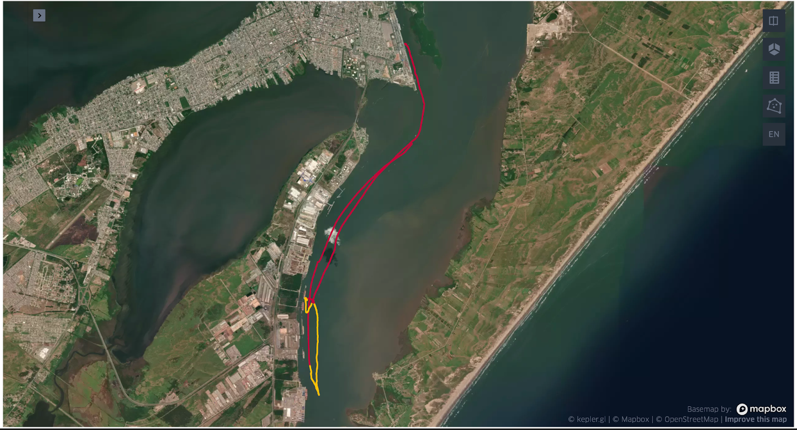
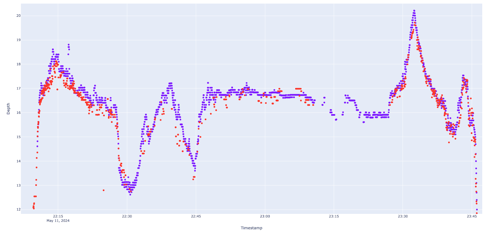
Throughout May 2024, we compared (Figs. 1–3) the daily depth data from each vessel against the reference RTS. This comparison allowed us to identify consistent trends of change, which we plotted on a single map to highlight areas of deposition and erosion. While noise is an inherent challenge, observing similar trends across different vessels over time provides strong indicators for the port to monitor these changes closely.

3.2 Emergency monitoring operations
Although DockTech provided continuous monitoring of the main channel, the pilot vessels reported signs of siltation in the entrance channel, particularly during maneuvers with heavy ships. Adverse weather conditions prevented traditional hydrographic surveys, leading the port to commission DockTech and WilsonSons to conduct an emergency survey.
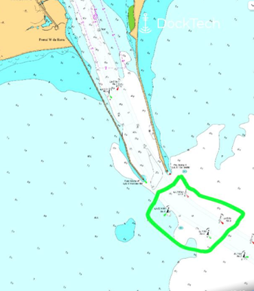
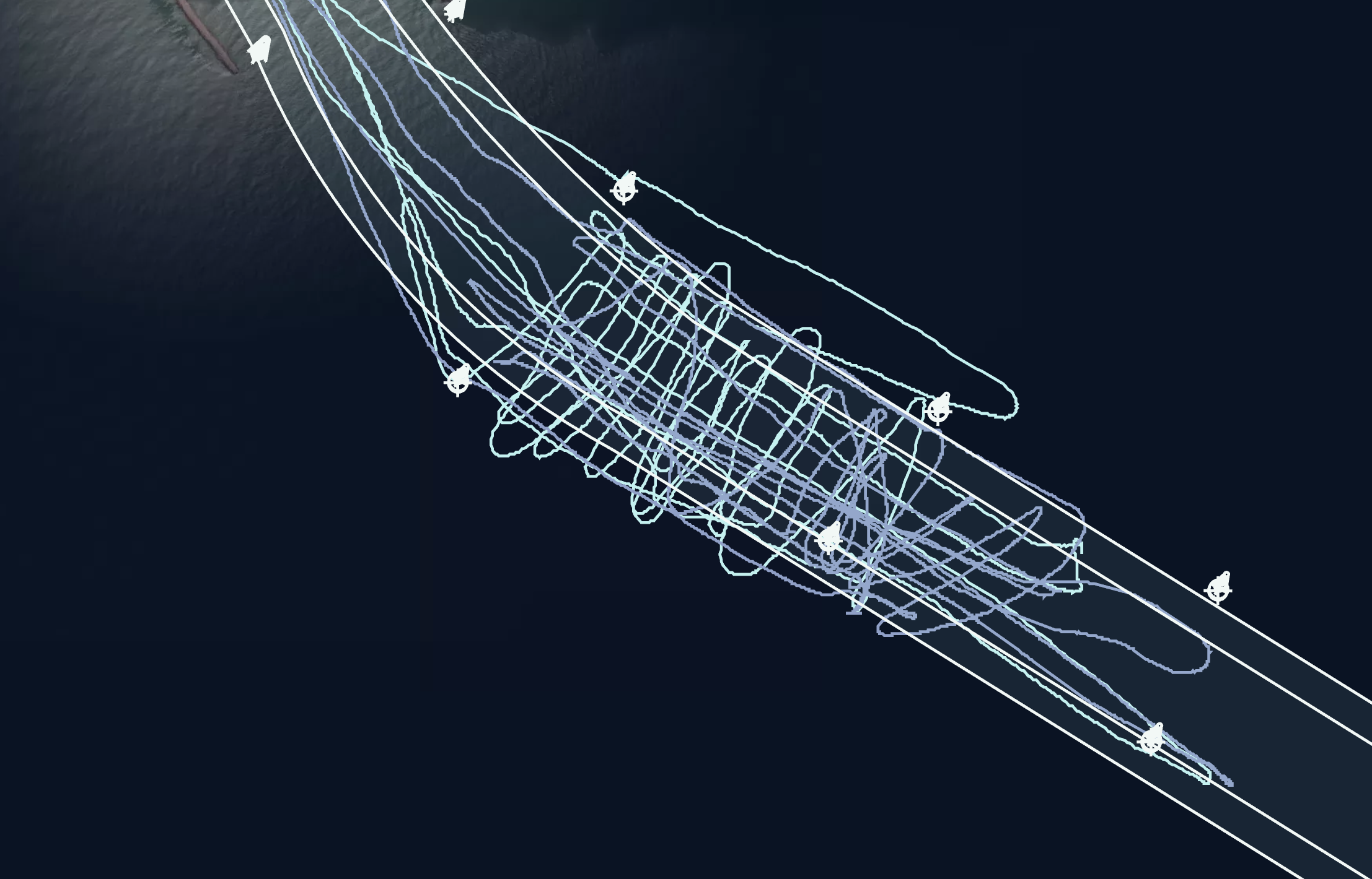
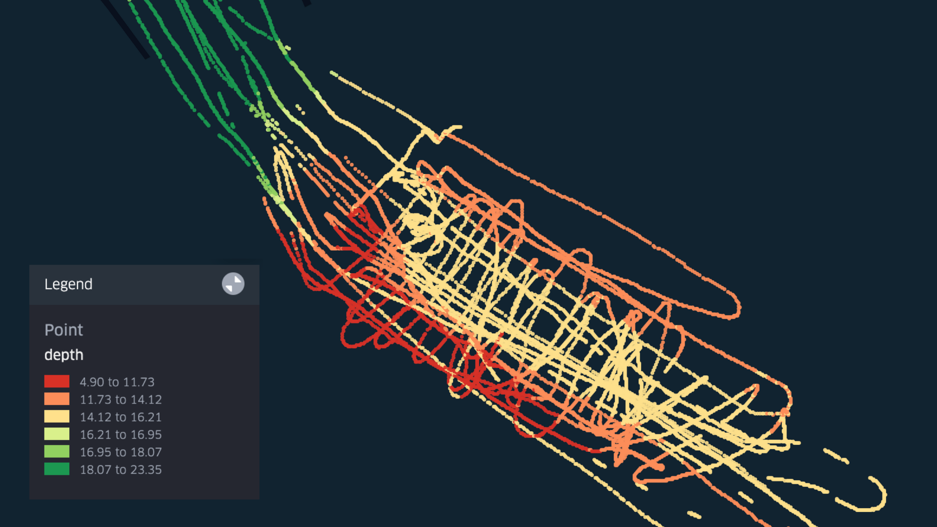
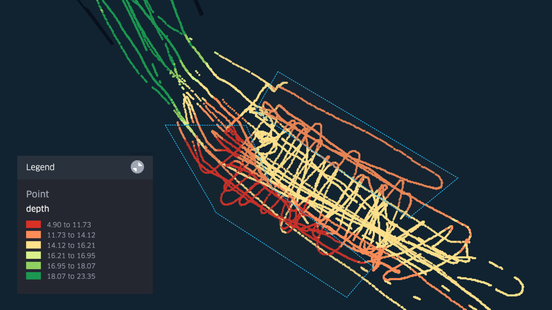
On June 6th and 7th, two tugboats from the fleet were deployed to map the entrance channel (Fig. 4). These vessels operated for approximately 1.5 hours each day, sailing in a criss-cross overlapping pattern (Fig. 5) at speeds below 10–12 knots. Tidal data was collected from the nearest tide station to the entrance channel, Molhe Sul. Tidal station data was vital because the observed water level raised more than a meter at the entrance of the port, compared to astronomical predictions.
4 Data analysis
4.1 Daily data collection and analysis
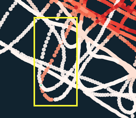
Every day the depth data (once filtered and enriched with tide and vertical offsets) from the past 24 hours are compared with the reference data (similar to Figs. 1 and 3). Depth difference is calculated and smoothed. Continuous observations of similar depth difference are clustered together. While a single cluster of difference might be a product of noise, as we compare the clusters generated across time and across vessels, larger trends become noticeable and confidence increases.
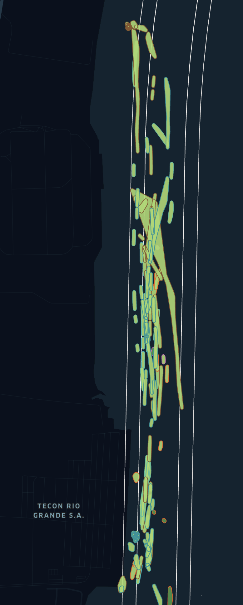
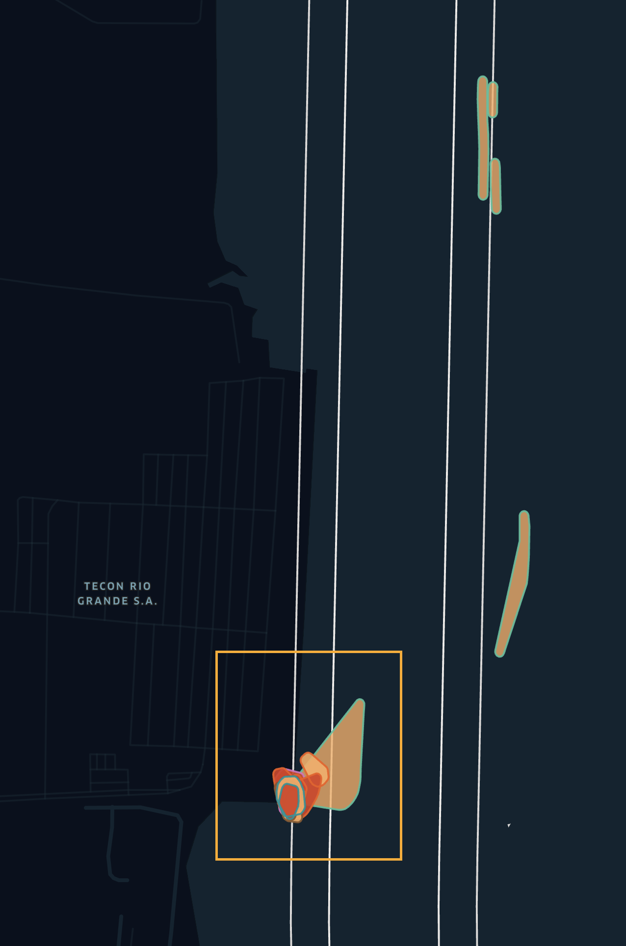
Below are two screenshots illustrating the trend polygons: erosion-only polygons (Fig. 6) and deposition-only polygons (Fig. 7). As shown, most of the main channel exhibits deposition. Erosion polygons, however, are limited to two areas: where the tugboats are berthed and along the eastern edge of the channel.
When we shared this information with the port authorities, they confirmed that these patterns of erosion and deposition were consistent with those observed in previous years, albeit on a smaller scale. This confirmation provides confidence that operations in the main channel can continue as usual, with a recommendation to avoid the eastern parts of the channel when possible.
4.2 Emergency monitoring operations
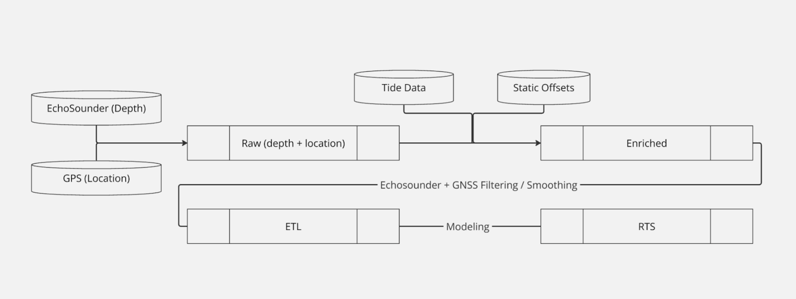
The pipeline (Fig. 8) running the code operates end-to-end without direct human involvement. Consequently, within a half-hour of the on-demand dredging operation, the results were available on DockTech’s app, Aquascope AI.
An immediate use case for the mapping was to identify the best possible entrance for a large shipping container with a draft deeper than the restrictions allowed. Using the general map (Figs. 9 and 10) we identified the shallower regions of the entrance channel. The pilot used this information in their decision-making process, successfully navigating the container vessel to the desired terminal.
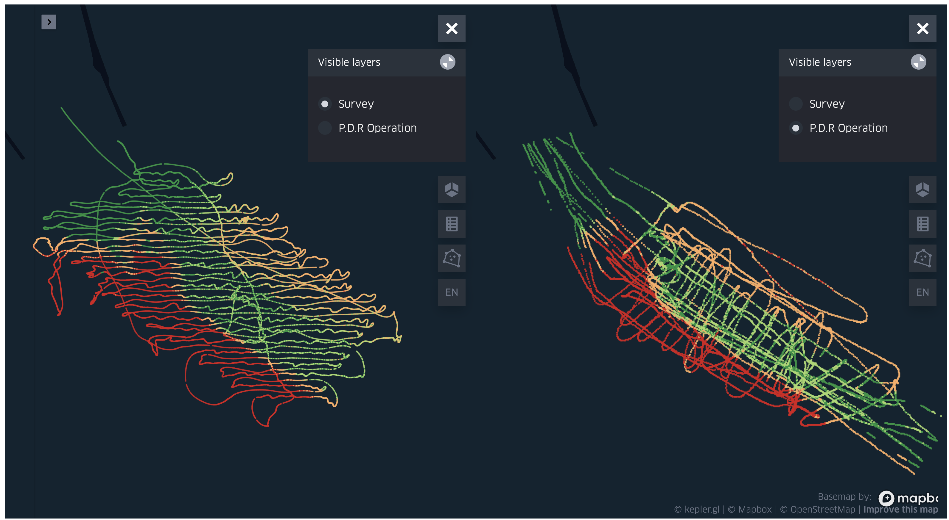
Two weeks later, the port conducted a traditional hydrographic survey using single-beam echo-sounder equipment. We compared our depth map to theirs, and while the ranges between the two layers are off by about a meter ([7.38, 21.39] for the survey, and [8.74, 22.88] for our layer), we can visually identify that the relative changes in the port are persistent (Fig. 11).
For each of the two layers, we binned the depth into the four quartiles ([[0, 0.25), [0.25,0.5), [0.5,0.75), [0.75,1.0]] and for each bin assigned a color (Table 1).
Despite some small pockets of noise in the PDR operation, the overall trends are clearly captured.

5 Data quality
5.1 Preface
When discussing the quality of the data, it is essential to establish a few key points.
Distinction of terms – The distinction between terms like precision, accuracy, and uncertainty has been well-documented (Heiskanen & Moritz, 1967; IHO, 2022a). Here, we will reference these distinctions without delving into detailed explanations. It is important to note that while there are many potential steps needed for correction/calibration (IHO, 2005), for simplicity we focus exclusively on the final output data.
Accuracy – To validate accuracy, we require some form of external validation (e.g., traditional surveys).
Precision – To validate precision/consistency, we can rely on the internal consistency of the data itself, both per vessel and across vessels. We compare measurements in the same location from various times and vessels.
If we have high accuracy (with low variance) we have confidence in our estimations as to accurately predicting the seafloor. If we have high precision, even with low accuracy, we can’t trust a particular reading, but we can rely on changes to reflect trends.
5.2 Daily data collection and analysis
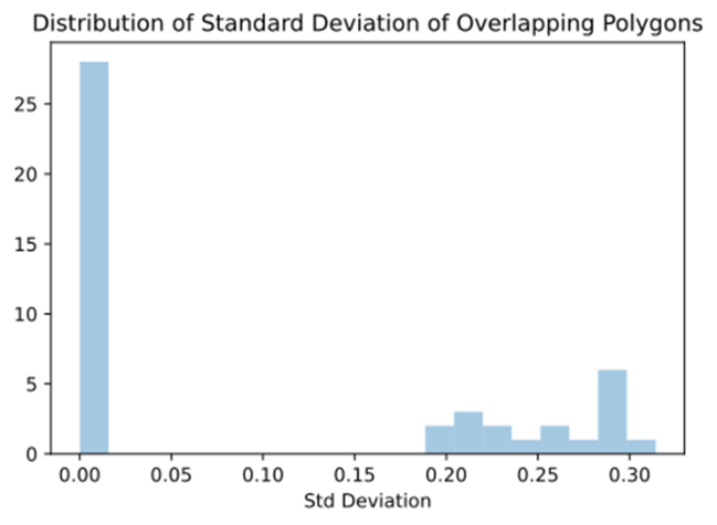
As we aim to capture daily change trends in a region with high uncertainty, we lack an external validation mechanism to evaluate the accuracy of our model. However, to estimate precision and consistency, we can examine the trend polygons generated (Figs. 6 and 7). By comparing overlapping polygons (demo example Fig. 12) and evaluating the depth differences, we derive the plot below (Fig. 13). These polygons were assessed over six days (May 16 to May 21).
Although capturing overlapping polygons precisely is challenging, the samples we have (n=46) show that the polygons are generally quite similar, with consistent trends even in cases with higher standard deviations.

5.3 Emergency monitoring operations
Because the vessels overlapped in their operations, we can calculate the precision of the model by evaluating the consistency (standard deviation) of the cells over time.
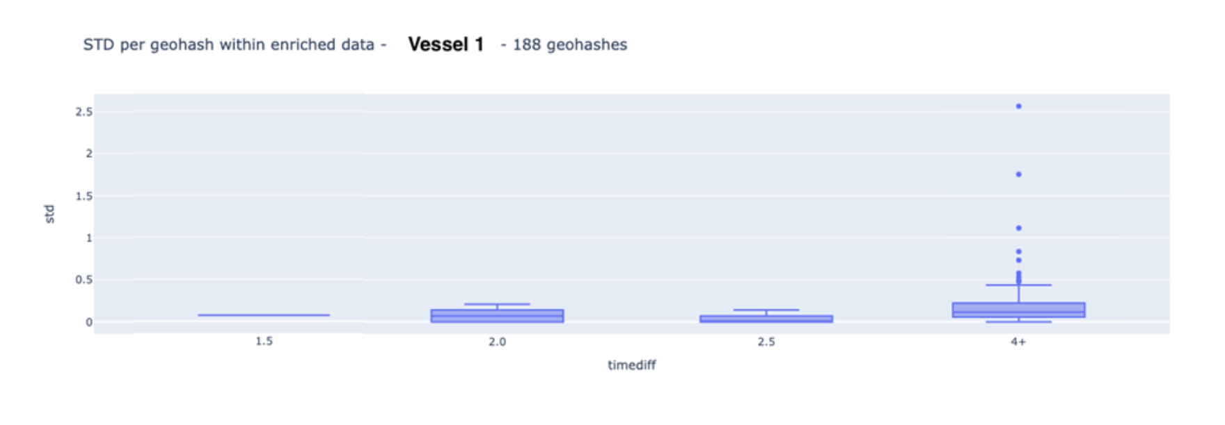
In most of our vessels we have observed a sampling frequency of two seconds for the depth data. In our particular use case, one of the two vessels has a sampling frequency of one second. As our cells are approximately 5 m × 5 m (geohash precision 9; Fox et al., 2013), we often have two subsequent readings per cell (when vessels go slower than 4.86 knots). To better understand precision, we created a boxplot per vessel, with the X-axis representing the time interval between measurements. The plots below (Figs. 14 and 15) show that while there are outliers (noise) causing internal variance per cell to exceed 50 cm, 95 % of the standard deviation is within 25 cm, and 98 % is within 35 cm.

Upon direct examination of the data, we did not observe traditional noise (e.g., shallow readings from fish or air bubbles), but we did identify an interesting phenomenon (Figs.16 and 17):
- Depth observations in relation to neighboring points indicate noise.
- Despite the vessel’s movement, the depth remained constant for half a minute before abruptly changing by over four meters.
Due to the port’s immediate need for results, we did not filter out any of the noise. As the primary goal was to track general trends, any minor noise could be empirically identified and ignored.
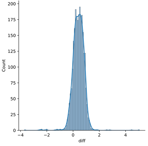
When comparing our RTS data to the survey data collected (Fig. 9), we plot the error histogram (Fig. 18). Since the hydrographic survey occurred two weeks later, we cannot simply treat the survey as “ground truth”. Due to constant sediment transport, bathymetric surveys are, by definition, only accurate at the time of collection. Normally, this is not an issue, as sediment transport does not change drastically. However, in our case, since the situation occurs at the end of a flooding event, additional debris deposition is expected. Nevertheless, we can still assess the overall quality of our data.
Overall, we see a mean error of around 40 cm, with a standard deviation of around 42 cm.
- Overall the residual error looks gaussian, which allows us to more easily define Confidence Intervals and Accuracy of the data.
- It is unclear what the mean error comes from. A shift from the mean error has often come from using inaccurate water level/tidal data or static offsets (echosounder to water level offset). In this scenario, in-situ tidal measurements were used and offsets were validated with blueprints. One speculation is the dynamic draft that is not yet being counted for, however as there are potentially other sources of error (e.g. speed of sound), further investigation is needed.
- Even with the mean error, as the spread is not too significant (± 2m fits within S-44’s Special Order; IHO, 2022b), the internal consistency of the port allows us to ensure that we can capture regions with general trends decently.
- We can also observe clear outliers, with depth difference values near ± 4 m. This would demand extra precautions if used to assist navigational maneuvering, but for the sake of trend detection, they are inconsequential.

Conclusion
As the port of Rio Grande in Brazil experienced a once-in-a-century flooding event, existing hydrographic surveys became unreliable, necessitating the implementation of a CSB-centric solution to detect trends and identify areas to avoid.
It is important to emphasize that CSB is intended to complement, not replace, traditional bathymetric surveys. The two use cases presented demonstrate how this approach can effectively identify trends in seafloor changes and provide clear guidance on navigation risks. While the second case may not fully align with the B-12 definition of CSB, the insights generated are theoretically achievable in a comprehensive CSB framework.
The application within the port of Rio Grande was crucial in allowing the port to safely reduce draft restrictions. This case study underscores the potential of CSB-equipped vessels as a dynamic and responsive tool in crisis management, offering valuable support during natural disasters.
References
Fox, A., Eichelberger, C., Hughes, J. and Lyon, S. (2013). Spatio-temporal indexing in non-relational distributed databases. 2013 IEEE International Conference on Big Data, Silicon Valley, CA, USA, 2013, pp. 291–299. https://doi.org/10.1109/BigData.2013.6691586.
Grinker, B., Solomon, S. and Hassin, A. (2022). Evaluation of a crowd sourced bathymetric approach. The International Hydrographic Review, 28, pp. 158–171. https://doi.org/10.58440/ihr-28-a08
Hains, D., Keating, S. G., Rathnayake, C., Obura, V., Sharma, S. and Hall, S. (2024). Citizen Hydrospatial Sciences − To csB or not to csB, that is the question! The International Hydrographic Review, 30(1), pp. 162–170. https://doi.org/10.58440/ihr-30-1-n02
Heiskanen, W. A. and Moritz, H. (1967). Physical Geodesy. W. H. Freeman and Company, San Francisco.
IHO (2005). Manual on Hydrography (1st ed.). IHO Publication C-13, International Hydrographic Organization, Monaco. https://iho.int/uploads/user/pubs/cb/c-13/english/C-13_Chapter_1_and_contents.pdf (accessed 3 October 2024).
IHO (2022a). Guidance to crowdsourced bathymetry (3rd ed.). IHO Publication B-12, International Hydrographic Organization, Monaco. https://iho.int/uploads/user/pubs/bathy/B_12_CSB-Guidance_Document-Edition_3.0.0_Final.pdf (accessed 3 October 2024).
IHO (2022b). Standards for Hydrographic Surveys (6th ed.). IHO Special Publication S-44, International Hydrographic Organization, Monaco. https://iho.int/uploads/user/pubs/standards/s-44/S-44_Edition_6.1.0.pdf (accessed 3 October 2024).
Jencks, J. and Jimenez Baron, B. (2024). CSB as part of the modern hydrographic toolbox. The International Hydrographic Review, 30(1), pp. 150–160. https://doi.org/10.58440/ihr-30-1-n03
Klemm, A. R. (2023). Introduction to Crowdsourced Bathymetry: The Power of Community. Medium. https://medium.com/@anthony.klemm/introduction-to-crowd-sourced-bathymetry-the-power-of-community-ad941ac20469 (accessed 3 October 2024).
Masetti, G., Rondeau, M., Jimenez Baron, B., Wills, P., Petersen, Y. M. and Salmia, J. (2020). Trusted Crowd-Sourced Bathymetry – From the Trusted Crowd to the Chart. A whitepaper jointly prepared by Danish Geodata Agency and Canadian Hydrographic Service. https://eng.gst.dk/media/9079/trusted-crowd-sourced-bathymetry-from-the-trusted-crowd-to-the-chart20200621.pdf (accessed 3 October 2024).References