1 Introduction

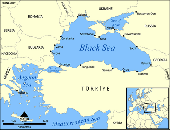
Recent military, political, and economic developments in the Black Sea region (Fig. 1) underscore the urgent need for a deeper understanding of the basin’s nature and mechanisms. The tempo-spatial variation of the Black Sea is of critical importance, particularly for operational purposes in navigation, security, and resource management (MacFarlane, 2024; Kılıçer & Kök, 2024).

This research primarily focuses on obtaining a comprehensive dataset concerning the geostrophic velocity anomalies of the Black Sea. The objective is to analyze the tempo-spatial variations and identify recurrent patterns in the surface currents by applying sophisticated clustering algorithms.

Self-Organizing Maps (SOMs) were specifically chosen for this study due to their high accuracy and effective performance in pattern recognition. Despite their proven efficacy, SOMs are not used in the Black Sea region, presenting a novel application in this context.

The integration of advanced clustering algorithms with satellite data provides a robust framework for understanding the complex circulation patterns of the Black Sea. This approach not only contributes to the scientific knowledge of the region but also has practical implications for addressing the emerging challenges posed by recent geopolitical and economic developments (Amarouche & Akpinar, 2023).

Despite the steady advancement in data availability through both in-situ observations and remote-sensing techniques, there remains a significant gap in the efficient and consistent processing and usage of this data. It’s estimated that only around 1% of the immense amount of satellite imagery collected is ever seen or analyzed by humans. This is largely due to the sheer volume of data produced by thousands of satellites constantly capturing images of Earth. As a result, artificial intelligence and machine learning technologies are increasingly relied upon to process and analyze this data, allowing for the identification of key patterns without requiring human review for every image (Frazier & Hemingway, 2021; Petrou, 2024).

The potential wealth of information contained within these unprocessed images is immense. Remote-sensing data can offer unparalleled insights into various oceanographic, atmospheric, and terrestrial processes. However, the current bottleneck in data processing limits the ability to fully harness these insights for scientific and operational purposes. Advanced processing tools and algorithms, such as SOMs and other machine learning techniques, are increasingly essential to bridge this gap. These tools can automate the analysis of large datasets, identify significant patterns, and extract relevant features with high precision and efficiency.

In the context of the Black Sea study, the use of SOMs exemplifies the application of advanced neural network methods to overcome the challenges of data processing. By leveraging such techniques, researchers can maximize the utility of remote-sensing data, ensuring that a higher percentage of collected images are analyzed and utilized effectively. This approach not only enhances the understanding of the Black Sea’s tempo-spatial variability but also sets a precedent for similar studies in other regions.

Ultimately, addressing the inefficiencies in data processing will enable more comprehensive and accurate environmental monitoring and forecasting. By improving the tools and methods available for data analysis, we can better manage and interpret the vast amounts of information collected, leading to more informed decision-making and a deeper understanding of the natural world.

The SOM is introduced as a viable solution to bridge the ever-widening gap between available data and processed data. SOM, also known as the Kohonen map, is an unsupervised neural network method grounded in competitive learning principles (Kohonen, 1988). One of the most significant features of SOM is its ability to preserve the neighborhood relationships of high-dimensional input data while projecting it onto a lower-dimensional, preferably two-dimensional, space. This capability makes SOM a topology-preserving technique.

2 Study area

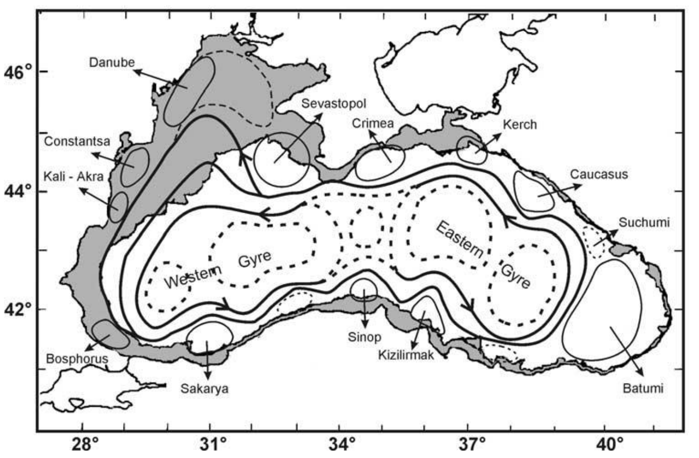
The Black Sea’s circulation is characterized by its dominant feature, the basin-wide cyclonic circulation known as the Rim Current, spanning 40–80 km in width. This distinctive circulation pattern is primarily driven by the mean cyclonic wind pattern prevailing in the region, coupled with the substantial input of buoyancy (Oguz et al., 1995). Notably, model simulations have underscored the crucial role of bathymetric data in sustaining the Rim Current; without incorporating bathymetry, the Rim Current diminishes significantly (Oguz et al., 1995).

Furthermore, model simulations have revealed that variations in wind stress, particularly weakening during spring and summer, lead to a reduction in the intensity of the mean current (Stanev, 1990; Grégoire et al., 2008). This decrease in intensity triggers intensified meandering of the Rim Current, particularly along the Turkish and Caucasian coastlines, giving rise to the formation of large meanders spanning 100–200 km. These meanders not only alter the flow patterns but also play a significant role in the redistribution of water masses and associated properties.

Satellite data analysis and hydrographic observations have provided further insights into the Black Sea’s circulation dynamics. Both data sources have confirmed the existence of recurrent, near-shore, anti-cyclonic eddies situated between the Rim Current and the coastline, alongside several cyclonic gyres within the central basin area (Oguz et al., 1992; Oguz et al., 1993; Oguz et al., 1994). These eddies and gyres contribute significantly to the local mixing and transport processes, influencing the distribution of heat, salt, and nutrients within the Black Sea.

The Black Sea’s circulation exhibits a rich tapestry of dynamical features, from the basin-wide Rim Current to the formation of meanders, eddies, and gyres along its coastline and central regions. These circulation patterns not only shape the physical environment of the Black Sea but also influence its biological productivity, ecosystem dynamics, and connectivity with adjacent water bodies (Fig. 2).

Understanding the complex interplay between these circulation features is essential for deciphering the Black Sea’s dynamics and its broader implications for regional and global oceanographic processes. By integrating observational data, model simulations, and remote-sensing techniques, researchers can gain a comprehensive understanding of the underlying mechanisms driving the Black Sea’s circulation and its response to external forcing factors.

Among these near-shore and anti-cyclonic eddies, two persistent eddies are noticeable: the Batumi Eddy and the Sevastopol Eddy. The interior part of the Rim Current, on the other hand, is composed of detached cyclonic gyres. These detached cyclonic gyres consist of either one gyre located in the eastern part of the sea and the other located in the western part of the sea, or a single extended cell dominates the basin. The scales of the central gyres and eddies vary from tens to hundreds of kilometers. Inter-annual variability of the Black Sea circulation is significantly affected by river discharges, local dynamics, and wind forcing’s seasonal variability (Stanev et al., 1995). Mesoscale, seasonal, and inter-annual variability was best described by the observations made by satellite altimeters (Stanev et al., 2000).

3 Data

The AVISO project plays a pivotal role in advancing our understanding of ocean dynamics through the systematic collection, validation, and interpretation of satellite-derived oceanographic data¹ (Ducet et al., 2000). Initiated with the aim of harnessing the wealth of information provided by satellite observations, AVISO serves as a comprehensive repository for oceanographic data, facilitating global-scale studies on ocean circulation, sea level variations, and related phenomena.

By collating data from a network of satellite missions equipped with altimeters and other remote-sensing instruments, AVISO provides researchers with a rich source of high-quality data spanning diverse spatio-temporal scales. The project employs rigorous validation procedures to ensure the accuracy and reliability of the collected data, enabling scientists to analyze and interpret oceanographic processes with confidence.

Moreover, AVISO offers valuable tools and resources for data visualization, analysis, and model validation, fostering collaboration and knowledge exchange among the global oceanographic community. Through its user-friendly interface and comprehensive data archives, AVISO facilitates interdisciplinary research efforts aimed at addressing key scientific questions related to climate variability, ocean circulation, and marine ecosystems.

The geostrophic velocity data from 1992 to 2012 were obtained from AVISO to provide data on the surface currents. Different time frames were selected and examined throughout the initial analyses. A ten-year-long data set was found to be sufficient when extracting the patterns of the long-term temporal and spatial variation due to the fact that any data sets covering a period longer than 10 years do not affect the results. Therefore, this research focuses on data sets from 1999 to 2009.

4 Methodology

In this study, the extensive dataset provided by the AVISO project is leveraged to investigate the tempo-spatial variability of the Black Sea surface circulation. By combining satellite-derived data with advanced analytical techniques, such as SOMs, it’s aimed to uncover recurrent patterns and dynamics within the Black Sea, shedding light on its complex oceanographic processes and their interactions with larger-scale climatic phenomena.

The methodology involves the detailed examination of satellite-derived data from the Archiving, Validation, and Interpretation of Satellite Oceanographic data (AVISO) project. By applying SOMs, classification, and interpretation of the variability in surface circulation is aimed to help providing valuable insights into the dynamical processes governing the region. The study then seeks to correlate these identified patterns with large-scale teleconnection indices, such as the North Atlantic Oscillation (NAO), the East Atlantic/West Russian (EAWR) oscillation, and the El Niño-Southern Oscillation (ENSO). Understanding these correlations is vital, as these indices significantly influence atmospheric and oceanographic conditions on a global scale.

4.1 ‘Learning’ in neural networks

Before we explore the learning capability of SOM, it’s crucial to establish a clear understanding of the concept of learning in neural networks. Learning can be conceptualized in two distinct ways: biologically and mechanically. Biologically, learning refers to the process through which an organism undergoes experiences that result in alterations to its state and enhance its performance in similar situations thereafter. In contrast, mechanical learning involves a computational approach aimed at achieving new intelligence and organizing this intelligence to acquire new abilities (Noyes, 1992). Considering these definitions, it becomes evident that for a neural network to be deemed useful, it must possess the ability to learn. The training process of neural networks facilitates learning, enabling the network to acquire knowledge and adapt its behavior for practical applications (Mishra, 2024).

Another approach to categorizing the learning process involves considering the level of control over the data. In this context, two primary forms of learning emerge: supervised learning and unsupervised learning.

In supervised learning, the network is provided with accurately labeled data, and the objective is to train the network to produce corresponding outputs for given inputs. Both input and output vectors benefit from supervised learning. Once the output vectors are generated, they are compared with the expected outputs to assess the network’s performance and identify any discrepancies.

Reinforcement learning represents a specialized form of supervised learning wherein the network receives feedback solely on the accuracy of its outputs. This feedback mechanism is often implemented through back-propagation algorithms (Mishra, 2024).

In unsupervised learning, the availability of accurate answers beforehand is either limited or absent altogether. Unlike supervised learning, where accurate answers guide the training process, input vectors are handled independently in unsupervised learning. Output vectors play no role in the learning process. Instead, the network operates as a self-governing entity, tasked with autonomously extracting patterns from the input data without any external interaction, particularly human intervention. This autonomous feature is particularly valuable when dealing with large and complex datasets, where manual computation is impractical or infeasible due to time constraints or computational complexity.

Unsupervised learning serves as the foundation for methodologies such as self-organizing maps (Guthikonda, 2005), wherein the network autonomously organizes and represents the input data in a structured manner, revealing inherent patterns and relationships without the need for explicit supervision.

4.2 SOM

SOMs are first introduced by Tuevo Kohonen (Kohonen, 1988) and derive their name from their inherent ability to organize themselves autonomously, without the need for external supervision. SOMs employ competitive learning, enabling them to learn independently.

The term “maps” in SOMs refers to their method of handling input datasets, wherein they endeavor to map the weights of the data. Nodes within the SOM network strive to mimic the characteristics of the input datasets they receive initially. This responsive behavior of the nodes forms the cornerstone of the entire learning process.

Central to the functioning of SOMs is the principle of preserving the essential characteristics of the input datasets. This principle distinguishes SOMs from other methods and underscores their significance. By retaining the topological relationships among the input data and mapping these relationships onto an SOM network, SOMs offer a valuable means of representing complex datasets (Guthikonda, 2005)

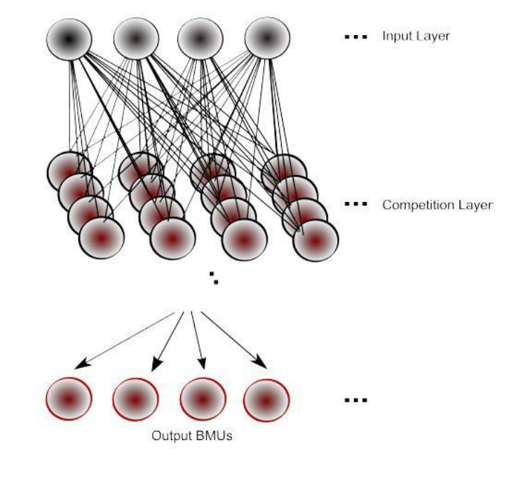
SOMs exhibit a relatively simple structure, with several noteworthy aspects. Fig. 3 illustrates a 4 × 4 SOM network, serving as the competition layer. Each input node establishes connections with every map node, resulting in a considerable number of connections even in small networks, such as the one depicted in Fig. 3 (e.g., 4 × 4 × 4 equals 64 connections). In contrast, there are no direct connections between map nodes within the network. The organization of nodes forms a two-dimensional grid, facilitating visualization of outputs and aiding in the implementation of the SOM algorithm. Each node in the network is assigned a unique coordinate (i,j), simplifying node referencing and range determination. However, it’s important to note that map nodes are unaware of the values held by their neighbors, as they solely interact with input nodes. Consequently, each node must rely on information from input vectors to update its weights.

The weight vectors of both the map nodes and the input vectors should match to enable the algorithm to perform properly (Mishra, 2004).

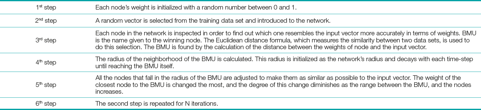
As an unsupervised learning algorithm, SOM has learning and prediction phases. During the learning phase, map is built; network organizes using a competitive process with a training set. During the prediction phase, new vectors are quickly given a location on the converged map, easily classifying, or categorizing the new data. The algorithm of the self-organizing map can be described as six main steps, which are presented in Table 1 in detail (Kohonen, 2013).

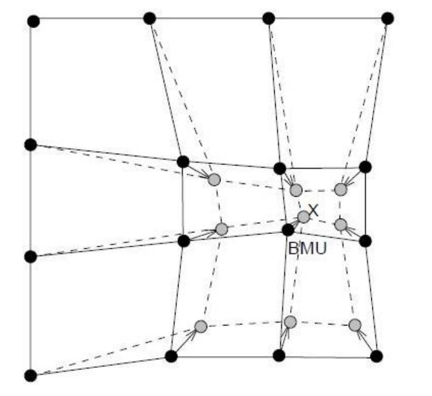
The degree of influence that the node’s distance from the Best Matching Unit (BMU) has on the node’s learning is shown by the influence rate. Initially, influence rate is set to 1 for all the neighboring nodes of the BMU and zero for the ones that are away from the BMU. At the end, due to weights’ random distribution and numerous iterations, SOM is able to settle down to a map of stable zones (Fig. 4), where nodes that do not fall into the neighborhood radius are entirely ignored (Kohonen, 2013).

The fact that the network is composed of nodes that are on a two-dimensional grid makes the calculation possible. The amount learned by the nodes on the edge of the neighborhood radius is a fractional value that is smaller than 1.0.

4.3 Davies-Bouldin index

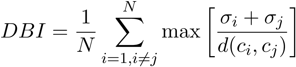
Davies-Bouldin index (DBI) is exerted to the data sets along with the SOM, to determine the number of patterns that best represents a data set. DBI was introduced by Davies et al. (1979) and is a measure that is used for assessing clustering algorithms.

(1)

DBI operates as an internal scheme, and the authentication of how precise the clustering has been accomplished is made using characteristics of the data set (Davies et al., 1979). In Eq. 1, N is the number of clusters, σ_i is the average distance of all patterns in cluster i to their cluster centers (c_i, σ_j) is the average distance of all patterns in cluster j to their cluster centers c_j, and d(c_i,c_j) is the distance between cluster centers c_i and c_j. Small values of DBI correspond to clusters that are compact, and whose centers are far away from each other. Consequently, the number of clusters that minimizes DBI is taken as the optimal number of clusters.

5 Results and discussion

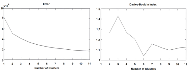
To study the temporal and spatial variation of the surface geostrophic velocities, the Black Sea basin is subject to iterative SOM analysis. The DBI demonstrates the best option with regards to the selection of total number of clusters to represent the whole data set. The smaller the DBI, the better and more practical the data representation is. Therefore, considering the DBI, the SOM analysis for the surface currents is based on six clusters (Fig. 5).

5.1 Six (spatial) patterns

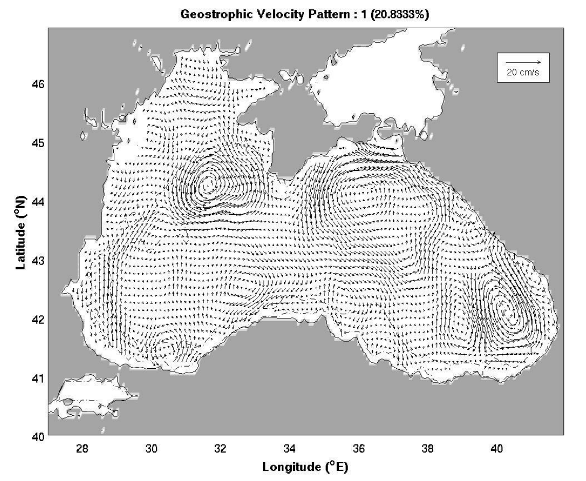
Pattern 1 (Sevastopol Cyclonic and Batumi Dipole Eddies):  The first pattern represents more than 20 % of the whole data set. In this pattern, the Batumi dipole eddies are detected at the southeastern corner of the basin. The eddy on the right is strong, cyclonic, and it spins at ~8 cm/s, whereas the other eddy is weak and anti-cyclonic. At the northwestern corner of the basin, the cyclonic Sevastopol eddy which spins at ~5 cm/s is evident. The general circulation is comprised of two main gyres. The western main gyre is anti-cyclonic and weak. The eastern main gyre, on the other hand, is cyclonic and strong. The northerly boundary current forms in the west. No eddy formation is observed in the open parts of the basin (Fig. 6).

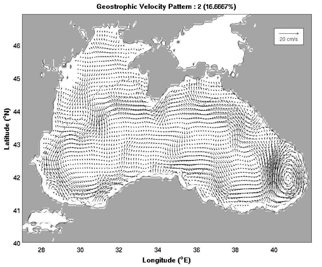
Pattern 2 (Cyclonic RIM Current and Anti-cyclonic Batumi Eddy):  More than 16 % of the data set is represented by the second pattern. The main feature of this pattern is the strong, anti-cyclonic Batumi eddy spinning at ~8 cm/s. Apart from the Batumi eddy, no other eddy structure, including the major Sevastopol eddy, is observed. The general circulation is formed by the strong and cyclonic RIM current flowing at ~5 cm/s. The basin’s open parts are relatively calm compared to the coastal regions. Therefore, this particular pattern is mostly dominated by the RIM current (Fig. 7).

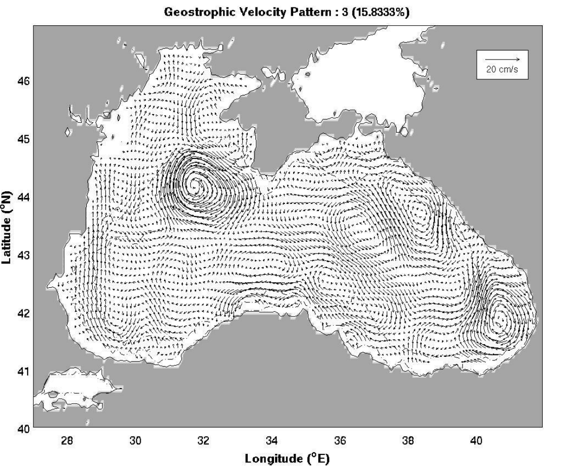
Pattern 3 (Anti-cyclonic Sevastopol and Batumi Eddies):  The third pattern represents almost 16 % of the whole data set. The major eddies of the basin are the Batumi and Sevastopol eddies which spin at ~7–8 cm/s. Both of these major eddies are strong and anti-cyclonic. The RIM current does not appear which means that the general circulation is formed by the western and eastern main gyres. The weak Caucasus eddy exists in the northeastern corner, while the strong northerly boundary current is present in the west (Fig. 8).

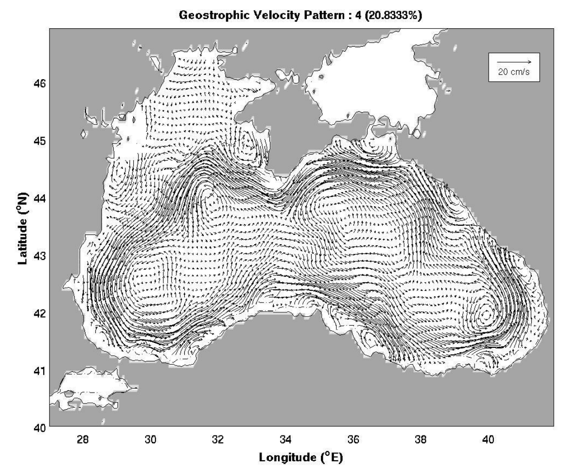
Pattern 4 (Cyclonic RIM Current and Batumi Eddy):  The fourth pattern comprises more than 20 % of the whole representation of the data set. In this pattern, the Black Sea basin is almost entirely dominated by the strong cyclonic RIM current which flows at ~10 cm/s. The open parts of the sea stay relatively calm, and the very weak cyclonic Batumi eddy is detected but it is nearly absorbed by the RIM current (Fig. 9).

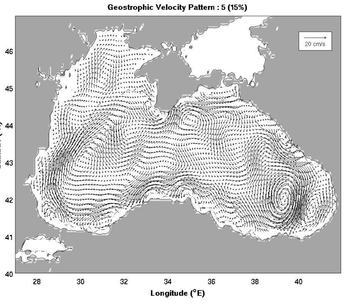
Pattern 5 (Anti-cyclonic RIM Current and Batumi Dipole Eddies):  The fifth pattern represents 15 % of the whole data set and it demonstrates a basin-wide, chaotic environment. At the southeastern corner the Batumi dipole eddies take place and the stronger eddy spins at ~7 cm/s. The weak, anti-cyclonic Crimea eddy is observed in the north, whereas the Sevastopol eddy disappears. The general circulation is formed by the strong, anti-cyclonic RIM current which flows at ~6–7 cm/s (Fig. 10).

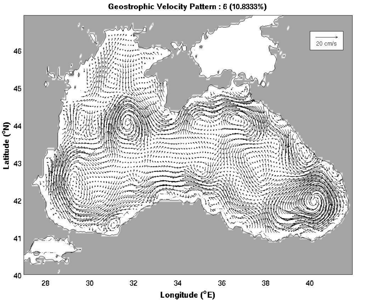
Pattern 6 (Anti-cyclonic RIM Current and Multi Eddies):  More than 10 % of the total representation for the data set is covered by the sixth pattern. The southeastern corner of the basin is entirely dominated by the strong, anti-cyclonic Batumi eddy spinning at ~8 cm/s. At the north of the Batumi eddy, the cyclonic Suchumi eddy is detected. The weak, anti-cyclonic Kerch eddy is observed in the north. At the northwestern corner the strong anti-cyclonic Sevastopol eddy forms, which spins at ~6 cm/s. The general circulation is comprised of the strong, anti-cyclonic RIM current (Fig. 11).

5.2 Temporal variation

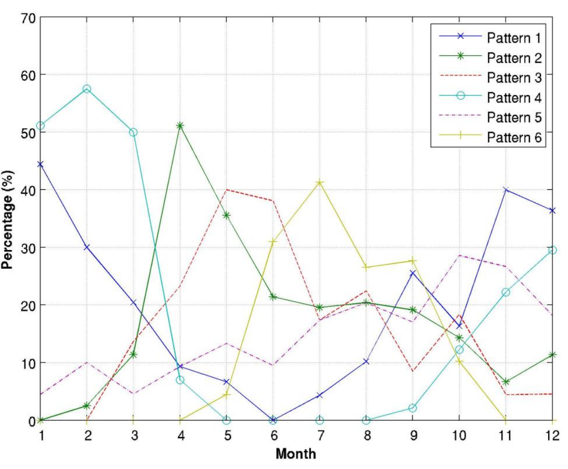
To better illustrate the monthly and seasonal variability of the surface currents, the rate of occurrence of the six patterns was computed and the results are shown in Fig. 12. Pattern 1 is one of the two patterns that dominates winter-like and fall-like months. Its maximum contribution is in January with ~45 % and it disappears completely in June. Even though there is less than 35 % chance it will appear, it is the pattern most likely to be observed in December. Pattern 2 is more likely to be observed during springtime. Its maximum contribution is detected in April with more than 50 % and it has the highest percentage among the six patterns in this particular month. In summer and fall it tends to stay at around 20 %, it declines in winter-like months, and it completely disappears in June. Pattern 3 tends to appear towards the end of spring and the beginning of summer. It reaches its maximum in May and becomes the pattern most likely to appear during that time of the year. It oscillates during fall-like months and never shows up in January and February. The first three months of the year are dominated by Pattern 4. It tends to appear strongly during cold periods, whereas during warm periods, it exhibits a weak contribution. Pattern 4 disappears in May and doesn’t appear again until September. Although Pattern 5 shows maximum percentages in fall-like months and dominates in October, it has no significant seasonality and occurs occasionally throughout the year. Pattern 6 completely disappears from November to April, appearing only five months during the year. It dominates the period from June to September and reaches its maximum in July. With more than 40 % contribution, it becomes the pattern most likely to be detected in July.

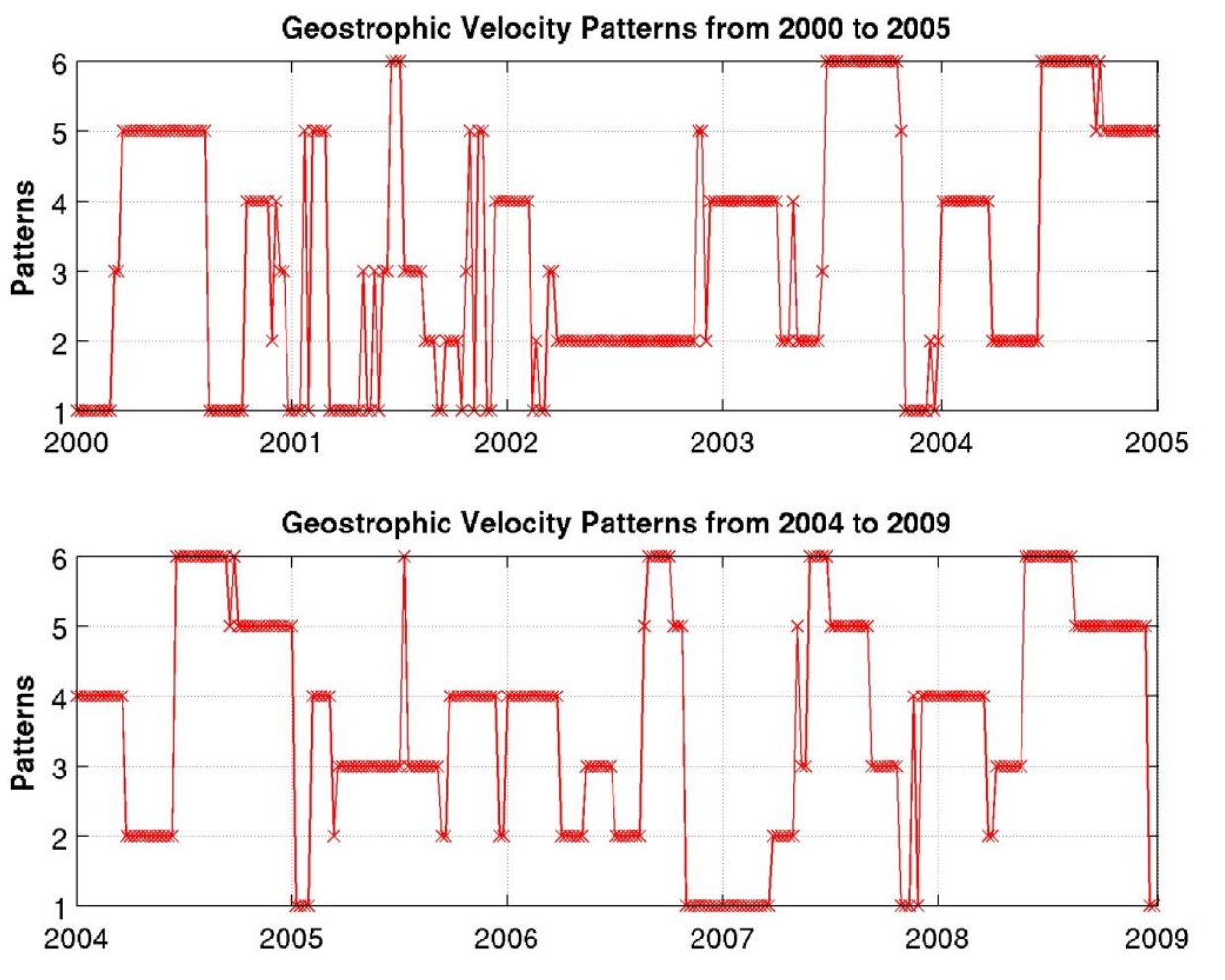
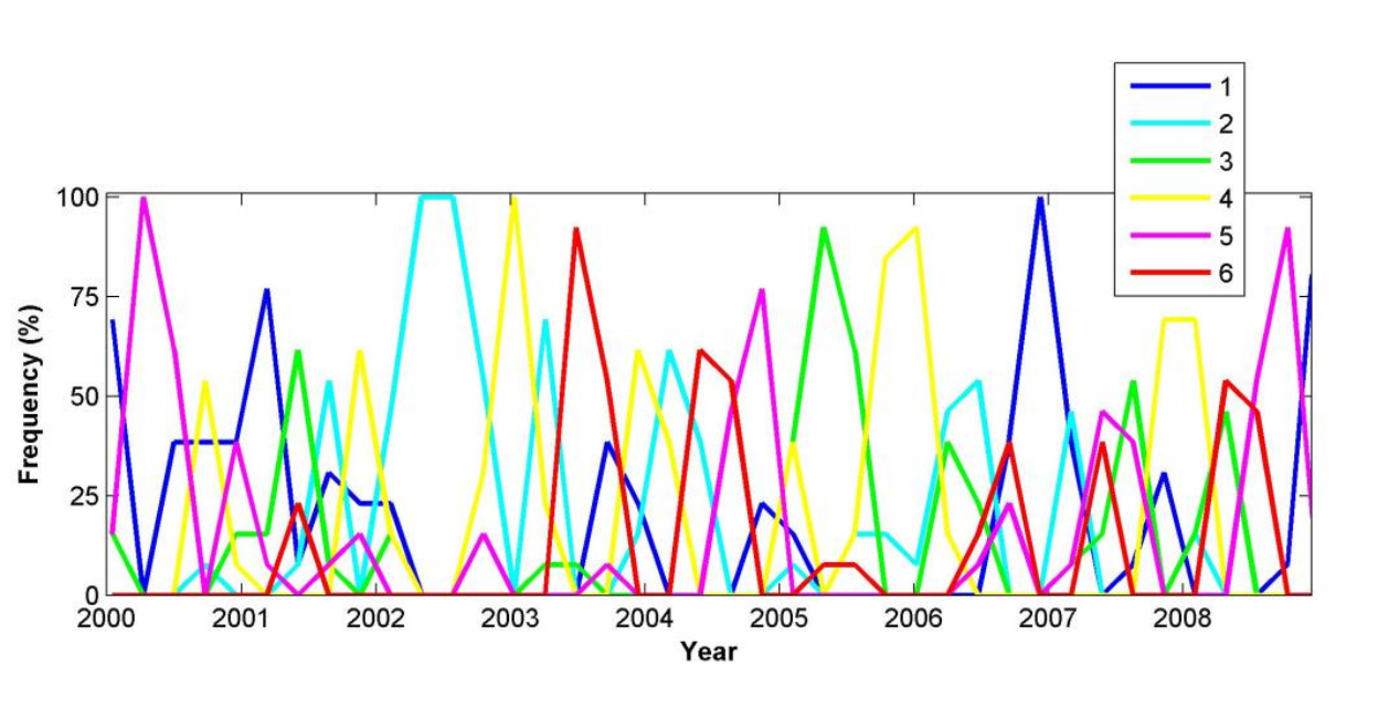
The time series of the six patterns of the surface currents from 2000 through 2009, with year 2004 overlapping, that was derived by SOM is shown in Fig. 13 and the evolution of the duration and the frequency of the same patterns is shown in Fig. 14 in order to illustrate the inter-annual variability.

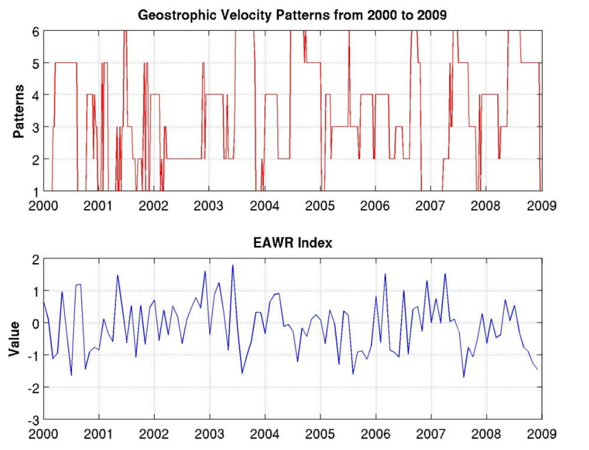
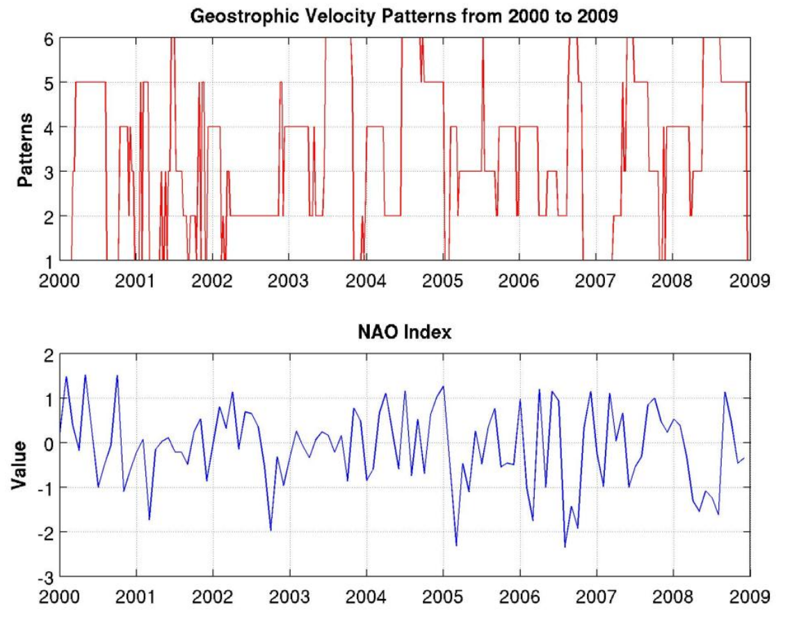
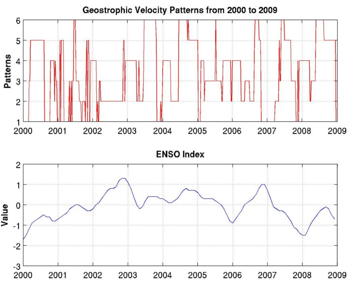
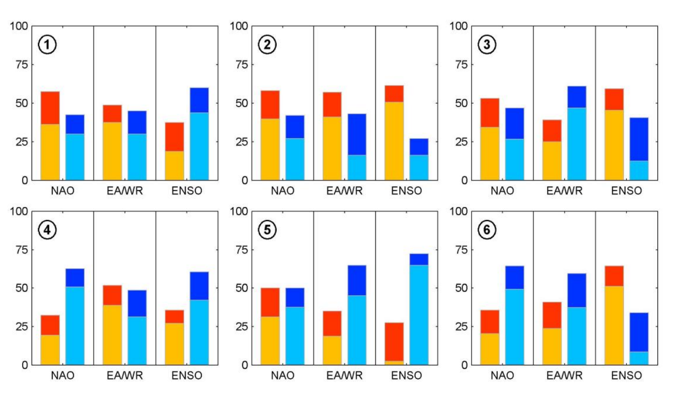
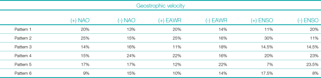
Furthermore, Figs. 15, 16, and 17 demonstrate the contemporaneous EAWR, NAO, and ENSO indices respectively, along with the times series of the surface currents. In addition to those figures, Table 2 is provided to allow a deeper understanding of the relationship between the surface currents and the large-scale teleconnection indices. The potential influence of large-scale teleconnection indices on the recurrent patterns of the surface currents (shown in Figs. 5–10) are evaluated by estimating for each recurrent pattern the value of the climate indices (i.e. EAWR, NAO, ENSO), acquired for different months mapped towards this pattern. This process enables determining whether a recurrent pattern is associated to either positive or negative value of a particular index significantly, and therefore a prospective connection between the surface currents over the Black Sea and large-scale teleconnection indices. Fig. 18 shows for each recurrent pattern of the surface current, the distribution of positive and negative phases of the three teleconnection indices. According to this figure, the EAWR index and the ENSO index are negative significantly during months mapped towards Pattern 5, which indicates that the occurrence of Pattern 5 (Anti-cyclonic RIM Current and Batumi Dipole Eddies) is promoted by the absence of these indices. On the other hand, ENSO index is significantly positive during months mapped towards Pattern 2 (Cyclonic RIM Current and Anti-cyclonic Batumi Eddy) and therefore influences the surface current structure.

6 Conclusion

Surface geostrophic velocity data from 1999 to 2009 were obtained from AVISO as the base dataset on the surface currents. Six patterns as to these velocities were found after conducting the SOM analyes. The inter-annual variability of the surface currents was also obtained.

The rate of occurrence of the six patterns was computed. Pattern 1 is one of the two patterns that dominates winter-like and fall-like months. Its maximum contribution is in January with ~45 % and it disappears completely in June. Pattern 2 is more likely to be observed during springtime. Its maximum contribution is detected in April with more than 50 %. It declines in winter-like months, and it completely disappears in June. Pattern 3 tends to appear towards the end of spring period and the beginning of the summer period. It reaches its maximum in May and becomes the pattern most likely to appear during that time of the year.

The first three months of the year are dominated by Pattern 4. It tends to appear strongly during cold periods, whereas during warm periods it exhibits a weak contribution. Pattern 4 disappears in May and does not appear again until September. Even though Pattern 5 shows maximum percentages in fall-like months and dominates in October, it has no significant seasonality and occurs occasionally throughout the year. Pattern 6 completely disappears from November to April and appears only five months during the year. It dominates the period from June to September and reaches its maximum in July. With more than 40 % contribution, it becomes the pattern most likely to be detected in July. The EAWR index and the ENSO index are detected significantly negative during months mapped towards Pattern 5, which indicates that the occurrence of Pattern 5 is promoted by the absence of these indices. On the other hand, ENSO index is detected significantly positive during months mapped towards Pattern 2 (Pattern 2 has the highest possibility to form among the six patterns at 25 %) and therefore influence the surface current structure. As the last example of the significant indications, Pattern 6 has the smallest possibility of occurring at only 8 % when the ENSO index is negative.

The topology-preserving nature of SOM ensures that similar patterns in the input data are mapped to neighboring regions on the output map. This characteristic offers a substantial advantage in pattern recognition and feature extraction from complex datasets. By clustering similar data points together, SOM facilitates the identification of underlying structures and trends within the data, which might otherwise be obscured in high-dimensional spaces.

In practical applications, such as the analysis of Black Sea surface circulation that is carried out in this research, SOM can efficiently handle large and complex datasets derived from satellite observations. It enables researchers to discern meaningful patterns and variations in the data, which are crucial for understanding the tempo-spatial dynamics of the region. The ability to visually represent these patterns in a two-dimensional map simplifies the interpretation and communication of results, making SOM an invaluable tool for both data analysis and decision-making processes.

Moreover, the application of SOM in this context highlights its potential to enhance the processing and utilization of remote-sensing data. By reducing the dimensionality of the data while preserving its intrinsic relationships, SOM allows for more efficient data processing and more accurate identification of key features. This not only maximizes the utility of the available data but also paves the way for more informed and effective environmental monitoring and management strategies. The integration of SOM into the data processing workflow addresses the critical challenge of managing large volumes of high-dimensional data. Its topology-preserving properties and ability to cluster similar patterns make it a powerful tool for extracting valuable insights from complex datasets, thereby bridging the gap between data availability and data utilization.

The research findings are expected to enhance predictive models and operational strategies for the Black Sea. By identifying the tempo-spatial patterns and their driving mechanisms, we can better anticipate changes in the basin’s dynamics. This, in turn, will support various operational activities, from maritime navigation to environmental monitoring and disaster response. The innovative application of SOMs in this region highlights the potential for advanced neural network techniques to offer new perspectives and more accurate analyses of oceanographic data.

Acknowledgements

I would like to offer my sincere gratitude to distinguished Professor Peter C. Chu, for his encouragement, scientific guidance, and instructions throughout the course of the research. This study would not have been this educational and exciting without his wealth of knowledge and motivation. I also want to express my heartfelt appreciation to Doctor Ming-Jer Huang for his support and sharing his expertise unconditionally.

References

Amarouche, K. and Akpınar, A. (2023). Long-term spectral wave climate in the Black Sea based on directional wave spectra. 21 February 2023, PREPRINT (Version 1) available at Research Square https://doi.org/10.21203/rs.3.rs-2596229/v1

Davies, D. L. and Bouldin, D. W. (1979). A Cluster separation measure. IEEE Transactions on Pattern Analysis and Machine Intelligence, 2, pp. 224–227. https://doi.org/10.1109/TPAMI.1979.4766909

Ducet, N., Le Traon, P. Y., Reverdin, G. (2000). Global high-resolution mapping of ocean circulation from TOPEX/Poseidon and ERS-1 and -2. J. Geophys. Res., 105(C8), 19477–19498.

Frazier, A. E. and Hemingway, B. L. (2021). A Technical Review of Planet Smallsat Data: Practical Considerations for Processing and Using PlanetScope Imagery. Remote Sens., 13, 3930.

Grégoire, M., Raick, C. and Soetaert, K. (2008). Numerical modeling of the central Black Sea ecosystem functioning during the eutrophication phase. Progress in Oceanography, 76(3), pp. 286–333. https://doi.org/10.1016/j.pocean.2008.01.002.2004

Guthikonda, S. M. (2005). Kohonen Self-Organizing Maps. Wittenberg University.

Kılıçer, A. and Kök, O. (2024). Is the Black Sea Already a NATO Sea? Atlântica, 5. https://doi.org/10.58867/DBYO3056

Kohonen, T. (1988). Self-Organization and Associative Memory. Springer-Verlag, ISBN 0-387-18314-0.

Kohonen. T. (2013). Essentials of the self-organizing map. Neural Networks, 37, pp. 52–65.

Korotaev, G., Oguz, T., Nikiforov, A. and Koblinskyet C. (2003). Seasonal, interannual, and mesoscale variability of the Black Sea upper layer circulation derived from altimeter data. Journal of Geophysical Research: Oceans, 108(C4).

MacFarlane, S. N. (2024). NATO and Black Sea Security. In K. Kakachia, S. Malerius and S. Meister (Eds.), Security Dynamics in the Black Sea Region. Contributions to International Relations. Springer, Cham. https://doi.org/10.1007/978-3-031-62957-0_5

Maung, P. P. (2012). Augmented Reality using a Neural Network. Ripon College

Mishra, V. (2024). Neural networks and deep learning: theoretical insights and frameworks. https://doi.org/10.61909/AMKEDTB022409

Noyes, J. L. (1992). Artificial Intelligence with Common Lisp: Fundamentals of Symbolic and Numeric Processing. D. C. Heath, Lexington, MA.

Oguz, T. V., Aubrey, D. G., Latun, V. S., Demirov, E., Koveshnikov, L., Sur, H. I., Diaconu, V. S., Besiktepe, S., Duman, M., Limeburner, R. and Eremeev, V. (1994). Mesoscale circulation and thermohaline structure of the Black Sea observed during HydroBlack ’91. Deep-Sea Research I, 41, pp. 603–628.

Oguz, T. V., Latun, V. S., Latif, M. A., Vladimirov, V. V., Sur, H. I., Markov, A. A., Ozsoy, E., Kotovshchikov, V. V., Eremeev, V. V. and Unluata, U. (1993). Circulation in the surface and intermediate layer of the Black Sea. Deep-Sea Research I, 40, pp. 1597–1612.

Oguz, T., La Violette, P.E. and Unluata, U. (1992). The upper layer circulation of the Black Sea: its variability as inferred from hydrographic and satellite observations. Journal of Geophysical Research, 97(C8), 12569–12584.

Oguz, T., Malanotte-Rizzoli, P. and Aubrey, D. (1995). Winds and thermohaline circulation of the Black Sea driven by yearly mean climatology forcing. Journal of Geophysical Research, 100(C4), pp. 6845–6863.

Petrou, M. (2004). Special issue – Pattern Recognition for Remote Sensing (PRRS 2002) Preface. Pattern Recognition Letters, 25, 1459, ISSN: 0167-8655.

Stanev, E. V. (1990). On the mechanisms of the Black Sea circulation. Earth-Science Reviews, 28(4), pp. 285–319. https://doi.org/10.1016/0012-8252(90)90052-W.1990

Stanev, E. V., Le Traon, P. Y. and Peneva, E. L. (2000). Sea level variations and their dependency on meteorological and hydrological forcing: analysis of altimeter and surface data for the Black Sea. Journal of Geophysical Research, 105 (C7), 17203–17216.

Stanev, E. V., Roussenov, V. M., Rachev, N. H. and Staneva, J. V. (1995). Sea response to atmospheric variability, Model study for the Black Sea. Journal of Marine Systems, 6, pp. 241–267.

Vesanto, J., Himberg, J., Alhoniemi, E. and Parhankangas, J. (2000). SOM toolbox for Matlab 5. Helsinki, Finland: Helsinki University of Technology.

1. https://www.aviso.altimetry.fr/en/home.html (accessed 12 October 2024).