1 Introduction

Aquatic vegetation plays a vital role in freshwater and marine ecosystems as the interaction between flora and fauna creates intricate systems susceptible to ecological changes. These systems correspond to interactions between different biological and physical processes, which shape the distribution of macrophytes population in the surveyed aquatic landscape (Lønborg et al., 2021; Coops et al., 2007; Carpenter and Lodge, 1986; Wood, 1963). Pronounced changes in submerged vegetation therefore lead to constant flux in species diversity and abundance, which becomes of importance for economic interests in water systems, as well as climate related analysis of ecosystem health (Yamasaki et al., 2021; Coops et al., 2007; Schmieder, 2004, 1995; Carpenter & Lodge, 1986). These changes can be observed through different remote sensing and in-situ measurements, where geometric differences in the vegetation can directly be monitored. Therefore, enhancing the analysis of remote sensing data through automation can greatly improve the understanding of climatic factors upon the ecosystem (Carpenter & Lodge, 1986; Lønborg et al., 2021).

Current state-of-the-art surveying is still in-situ measurements with extensive measuring campaigns exploring pre-selected areas (Lønborg et al., 2021). For those areas of interest, diver- or boat-based surveys are often deployed to collect biological samples, underwater images and annotate species distributions of the local vegetation in the selected transect or quadrant (Murphy et al., 2018; Zervas et al., 2018; Rowan & Kalacska, 2021; Lønborg et al., 2021). The data gathered during such field campaigns often constitute just a short temporal insight into a much larger and complex system and, due to the subjective interpretation by the diver, the observation is often difficult to reproduce. This limits the achievable accuracy apart from the high costs to deploy divers at a high frequency (Lønborg et al., 2021).

Another commonly used approach to analyze submerged vegetation on a larger scale is photogrammetry. For this, there are two commonly used systems: (i) satellite based remote sensing (Luo et al., 2016; Nelson et al., 2006; Mandlburger, 2022) and (ii) airborne imaging using high resolution, multi- and hyperspectral cameras. Techniques based on satellite images have the advantage of large aerial coverage and avoid the deployment of ground-borne teams across long surveys, resulting in cost and time efficient measurements compared to surveys of similar extent conducted by survey teams (Mumby et al., 1999). The down side of such measurements is the low spatial resolution, as most satellite images have a resolution of around 1 to 50 m (de Grandpr´e et al., 2022; Rowan & Kalacska, 2021). Considering that for most processes of interest, higher resolutions are crucial, this entails inaccuracies due to averaging the gathered data across large pixels (O’Neill & Costa, 2013; Ackleson & Klemas, 1987). The second option is using orthophotos and hyperspectral images, captured from either crewed or uncrewed aerial vehicles (Mandlburger, 2022). These images feature a much higher resolution, depending on the system used and the employed above-ground altitude of the airborne system. The compromise of high spatial resolution introduces a limitation of the spatial extent or prolongs the survey, as the altitude influences the field of view (Lønborg et al., 2021). The increased resolution, however, allows for detailed analysis of the vegetation distributions and provides indicative results on plant species, but provides limited insights on the structural component of the macrophytes population (Dierssen et al., 2021).

On-water remote techniques, such as boat-based hydroacoustic sensing methods (e.g. sonar), have been widely recognized in different areas of aquatic mapping (McCarthy, 1997; Sabol et al., 2002; Aleksandra et al., 2015; Mandlburger, 2022). The application towards vegetation detection in particular has seen substantial improvement in terms of spatial resolution due to the application of multi-beam sonar (Aleksandra et al., 2015; Held & Schneider von Deimling, 2019). Systems pioneered by RoxAnn (single beam) and Questor Tangent Corporation (multibeam), have introduced and improved the classification of seabed types. Both systems utilize a similar classification method, based on the recorded acoustic variables and relate to these measures such as roughness and hardness of the seabed (Schiagintweit, 1993; Serpetti et al. 2011). Such feature-based approaches can furthermore be applied to the automatic vegetation detection and can cover vast areas in acceptable time periods (Blondel, 2008).

The same applies to bathymetric LiDAR, where improvements in sensor technology and signal processing have overcome previous limitations (Mandlburger et al., 2023b). This has established LiDAR among the traditional approaches for mapping macrophyte populations in water ecosystems (Wagner et al., 2024; Calantropio et al., 2024; Mandlburger et al., 2023b). Furthermore, due to the rise of unmanned aerial vehicles (UAVs), the technology has become widely available enabling the implementation of those recent advances in practice (Espel et al., 2020). One of such advancements is the recent utilization of full waveform LiDAR (i.e., the availability of the complete temporal record of the returned echo pulse), which enables specifically tailored signal processing for bathymetric LiDAR, improving water surface detection and higher depth penetration (Schwarz et al., 2019). Overall, recent advancements have allowed users to not only capture detailed aquatic vegetation but furthermore create a basis for detailed data analysis, as a multitude of features can be extracted from the acquired point clouds (Mandlburger et al., 2023a). In this new type of data, one of the challenges is the classification of the acquired points into submerged terrain and vegetation, which can not sufficiently be achieved by established methods (Wagner et al., 2024). Consequently, research related to the development of new methods in the classification of macrophyte subtypes is of great importance.

For classification methods of both sonar and LiDAR that are based on recorded variables (features), for each measured point, feature selection plays a vital role. In general terms, a classifier transforms an input vector into an output of a single value, the classification (Domingos, 2012). Therefore, selection, transformations, and the overall dimension of the data influence the generated output (Bellman & Kalaba, 1959; Chen, 2009; Domingos 2012). Previous studies in both fields of LiDAR and sonar have addressed these challenges and introduced different approaches (Serpetti et al. 2011; Schi, 2021). In such recent results both general large feature space and manually selected feature approaches have been used to generate classifications of point clouds, where each approach has distinct advantages and challenges (Serpetti et al. 2011; Shi et al., 2021, Saputra & Radjawane, 2022). Single feature selection on one hand requires human supervision, while machine learning built on all features requires large amounts of data and training (Serpetti et al. 2011; García-Gutiérrez et al., 2015; Yang et al., 2020; Shi et al., 2021, Saputra & Radjawane, 2022).

Related scientific work has seen a large increase in the deployment of LiDAR across different fields related to geoscience over the last decade (Mandlburger et al., 2023b; Rowan & Kalacska, 2021; Lønborg et al., 2021). This is also the case for bathymetric applications, where LiDAR expanded from simple topographic modeling to capturing detailed structures of submerged aquatic vegetation (Wagner et al., 2024; Rowan & Kalacska, 2021; Mandlburger et al., 2020). While the use of infrared LiDAR is already a common tool in forestry and other terrestrial ecological research (Zhou et al., 2022; Michalowska & Rapiński, 2021; Koma et al., 2021), the use of LiDAR for aquatic ecosystems is still limited due to expensive initial costs, which applies to airborne data acquisition from both crewed and remotely piloted platforms. Furthermore, only recent advances in sensor technology, specifically the increase in spatial resolution (smaller laser footprints and higher scan rates) has enabled the detection of submerged objects beyond mere mapping of bathymetry (Mandlburger et al., 2023b; Lønborg et al., 2021). Therefore, many challenges such as vegetation classification in vegetated water bodies are still not entirely solved for bathymetric LiDAR. To overcome the challenges posed by bathymetric LiDAR, different methods have been presented over the last years ranging from unsupervised machine learning to LiDAR feature-based classification methods (Saputra & Radjawane, 2022; Amani & Mahdavi, 2021; Wagner et al., 2024). Each approach faces different challenges. While machine learning requires large annotated datasets, data driven approaches depend on the investigated area and the system used (Saputra & Radjawane, 2022; Wagner et al., 2024). Additional challenges arise in the evaluation of such methods as the lack of benchmark datasets does not allow for a general comparison to other methods and thus introduces obstacles in comparison of effectiveness (Calantropio et al., 2024). This further extends to the manual annotation in general, as manually labeled datasets are prone to differ if annotated by multiple experts (Calantropio et al., 2024; Zhu et al., 2019).

This study aims to improve the current state-of-the-art of vegetation detection via LiDAR bathymetry through the introduction of a new method for the classification of 3D point clouds. The method is based on working principles of single cell clustering, where groups of cells are classified and matched on the basis of genetic similarity, such as the genes extracted from the cells during RNA-sequencing (Luecken & Theis, 2019). Related methods in the field of sonar signal processing have used acoustic variables from multibeam backscatter in combination with Principal Component Analysis (PCA) to identify main characteristics and assign each data observation to a specific class (Schiagintweit, 1993; Preston, 2009; Serpetti et al., 2011; Held & Schneider von Deimling, 2019). Applied towards LiDAR data, this is equivalent to combine all measurements of the laser scanning setup into a high-dimensional dataset and group the points based on similarity of the recorded features through dimensional reduction and clustering. The difference in the proposed method and current state of the art classification is the usage of Uniform Manifold Approximation and Projection for Dimension Reduction (UMAP; Sainburg et al., 2021) instead of a standard PCA workflow. Through the application of UMAP in the dimensional reduction, points with close spatial proximity (in the 2D dimensionally reduced dataset) have a similarity of features in the initial high-dimensional dataset. This improves the extraction of points with similar features and thus enables vegetation classification based on geometric similarities.

The workflow described in this article extracts the submerged LiDAR point cloud using the surface-volume-bottom algorithm (SVB) by Schwarz et al. (2019). The extracted data can be seen as a high-dimensional dataset made up of features for each point and can be dimensionally reduced to a two-dimensional dataset with UMAP, which can be clustered by density-based clustering algorithms. The extracted clusters can then be grouped into vegetation and non-vegetation labels providing an automated classification of the point cloud. The aim of the study is to extend the bathymetric processing pipeline to match best practices in other areas of remote sensing applied to ecological monitoring such as forestry, where LiDAR has become a standard tool to survey large areas and track biological changes over time (Michalowska & Rapiński, 2021; Kumpumäki et al., 2015).

The article first introduces the dataset used for development and evaluation, together with the deployed pre-processing (Section 2). In Section 3, we describe the construction of the high-dimensional feature space and the clustering of the dimensionally reduced dataset. This includes an introduction into dimensional reduction techniques and the classification of the created macrophytes groupings. The results of the developed method are further compared to photogrammetric and manually annotated data (Section 4) and critically discussed in the light of state-of-the-art ecological research (Section 5).

2 Materials

2.1 Study area

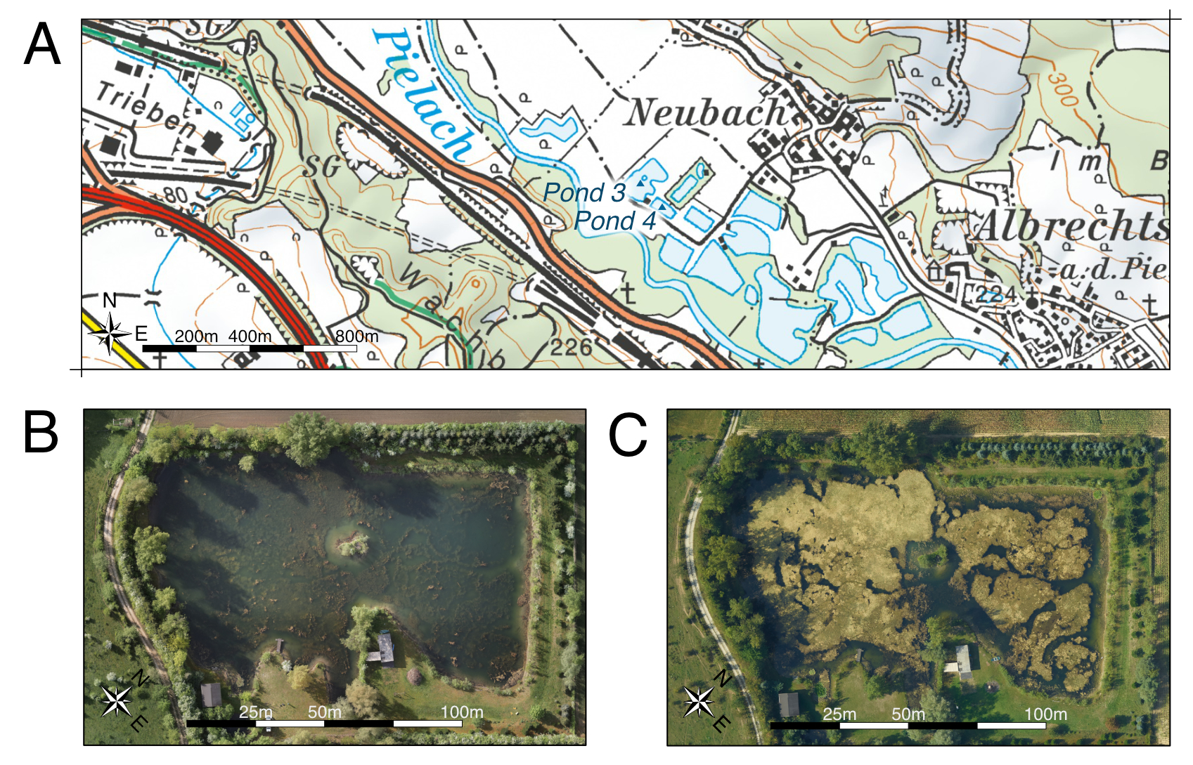
The study area is located near Loosdorf in the region of Lower Austria (48.2010 N, 15.4004 E; WGS 84). The entire region comprises a near-natural section of the pre-alpine Pielach river and around a dozen freshwater ponds in the adjacent flood plain. A subset of the ponds, including Ponds 2 and 3a, contain submerged vegetation, which can clearly be seen in the orthophotos obtained throughout multiple surveys (Fig. 1). This vegetation is under constant flux across the seasons and therefore representative of the general research related to the monitoring of submerged ecosystems. Furthermore, the combination of two different datasets (aerial images and LiDAR) provides a comprehensive foundation for post-analysis of the aquatic ecosystem.

2.2 Datasets

To capture the diverse landscape of submerged vegetation, two systems were deployed to generate a comprehensive dataset. First, the data was surveyed using a topo-bathymetric LiDAR system, in this case a RIEGL VQ-840-G topo-bathymetric UAV laser scanner system. The sensor was mounted on a helicopter and flown at an average flying altitude of 187 m, during a single day measuring campaign on the 9^th of February, 2022. The system uses a wavelength of 532 nm and medium sized footprints with an average footprint diameter between 0.82 m and 1.04 m (RIEGL, 2012, 2023). The data recorded by the LiDAR system was exported as a point cloud (Figs. 2a and 2b) in LAS format in a georeferenced coordinate system (ETRS89, UTM33; EPSG: 25833). Secondly, to capture reference data, standard photogrammetric methods were deployed to generate an orthophoto of the surveyed area (Fig. 2c). The orthophoto has a resolution of 5 cm per pixel based on images captured with a 12.4 MPix Manta G1236C camera mounted on the same helicopter setup as the LiDAR system. The orthophotos served as visual guidance for the annotation of the LiDAR point cloud, which has surface point densities of 34.4 points/m² and 27.4 points/m² for Pond 2 and 3a respectively.

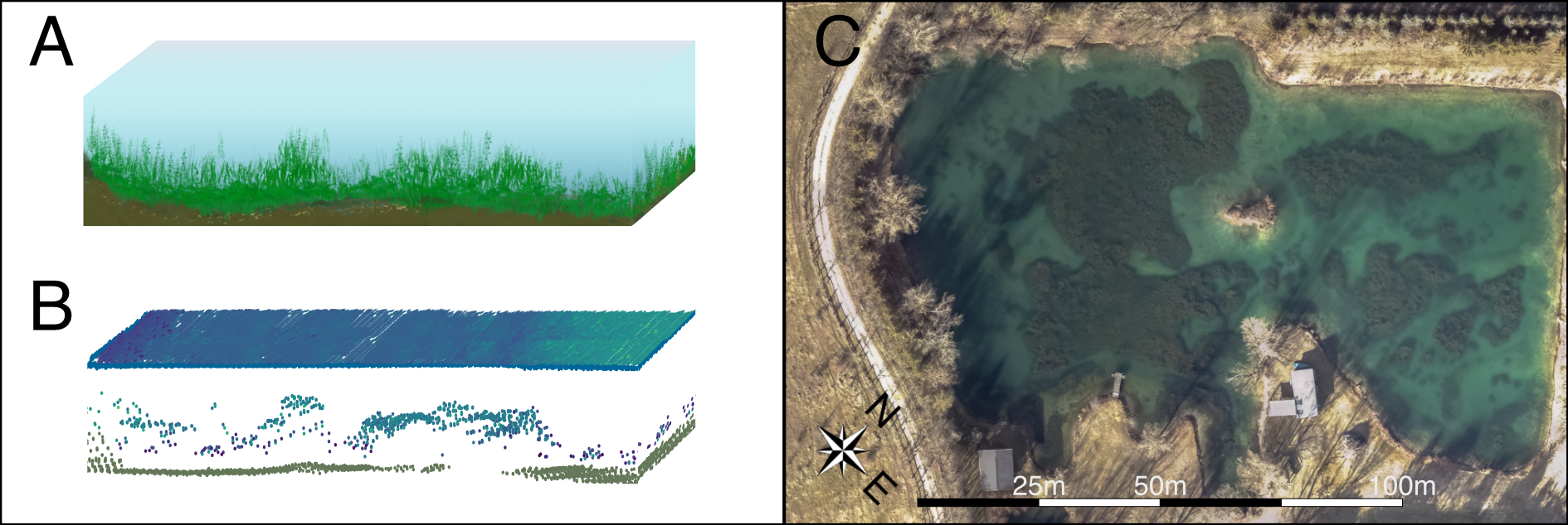
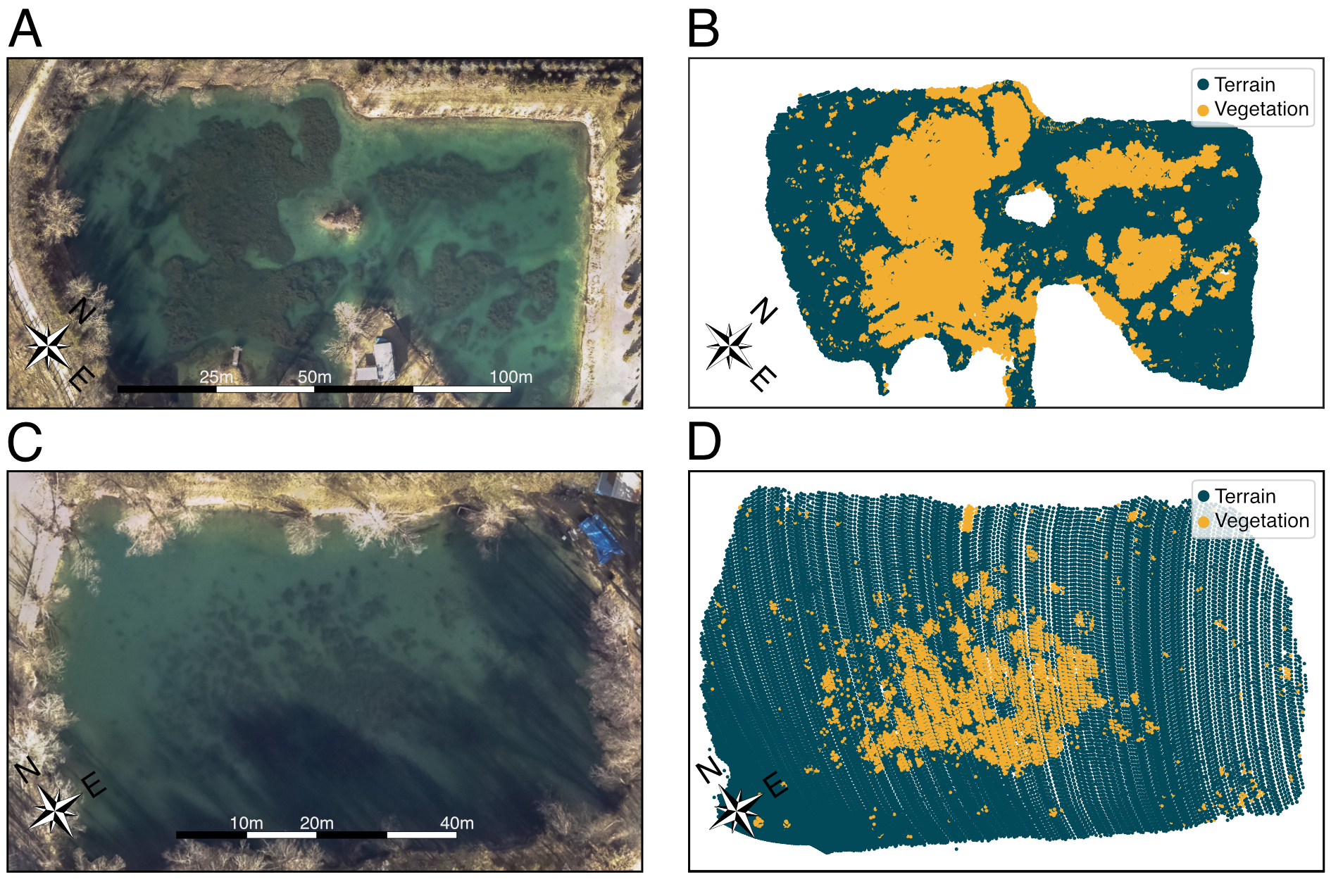
The first pond (Pond 2) features a variety of vegetation with different vertical extent and varying density (Figs. 2b and 2c). The second pond (Pond 3a) is considerably smaller, with an irregular vegetation distribution and many smaller patches. The labels are generated using the PointCloudLabeler¹add-on from OPALS version 2.6.0 (Pfeifer et al., 2014). This tool allows manual annotation of the point cloud in transects perpendicular to a digitized 2D axis (polyline). The transect is chosen so that the width covers the entire lake and the view-depth is set between 2 m to 5 m depending on operator preferences. The data were manually labeled by three experts. To avoid biases, the data were labeled twice by each expert, based on south-west and north-east oriented axis directions, respectively. In total, this resulted in six independently labeled data sets.

One of the challenges in the Pond 2 dataset is that the points are merged from two overlapping flight strips. The strip overlap area features higher point densities and varying distributions compared to the rest of the dataset. These differences are detectable throughout most of the features of the point cloud. To compensate for the artificial similarity of the features, we deploy point thinning in the overlap region. The thinning is based on an octree cutoff, reducing the number of points in the overlap to approximately match the rest of the point cloud. This leaves a final dataset comparable to the one of Pond 3a, which is only covered by a single flight strip. Together, both datasets are the input for the data processing (Section 3) and the final evaluation (Section 4).

2.3 Data preparation and water surface detection

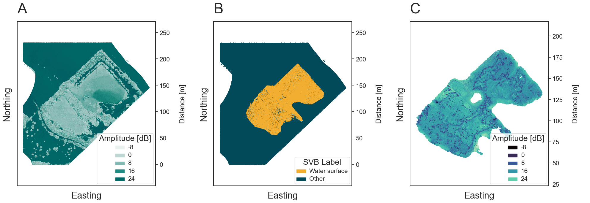
The data acquired by the topo-bathymetric LiDAR system captures all the features of the landscape, at land and underwater. To focus on the aquatic landscape, preprocessing of the data becomes necessary to remove all points not related to the submerged domain. For this, we introduce an initial step in the analysis that extracts the underwater area (Fig. 3c) from the recorded point cloud (Fig. 3a) by detecting the water surface within the study site and selecting only the points beneath the calculated water level. For this, we employed the SVB algorithm by Schwarz et al. (2019). The algorithm uses exponential decomposition of bathymetric laser waveforms (Schwarz et al., 2017), which provides a reliable classification of laser pulses hitting the water surface as a side product (Fig. 3b). From the initial identification of water surface points, the general water surface height in the respective coordinate system of the point cloud can be estimated. To select all points below the lowest part of the water surface, a threshold height is chosen based on the z-coordinate of all points classified as water surface, which fall in the range of the 2^nd–5^th percentile of the height. This accounts for potential outliers below the water surface. All points below the calculated threshold are expected to belong to the submerged area of interest. Lastly, to remove the remaining outliers, a simple clustering approach is applied to the data. Here, density-based clustering was chosen to remove all points not directly linked to the pond. In particular, we used DBSCAN (Pedregosa et al., 2011; Schubert et al., 2017; Ester et al., 1996), with a minimum distance of 1 m between the points. After this filtering step, the data is ready for further analysis, as only submerged terrain and vegetation remain (Fig. 3).

3 Method

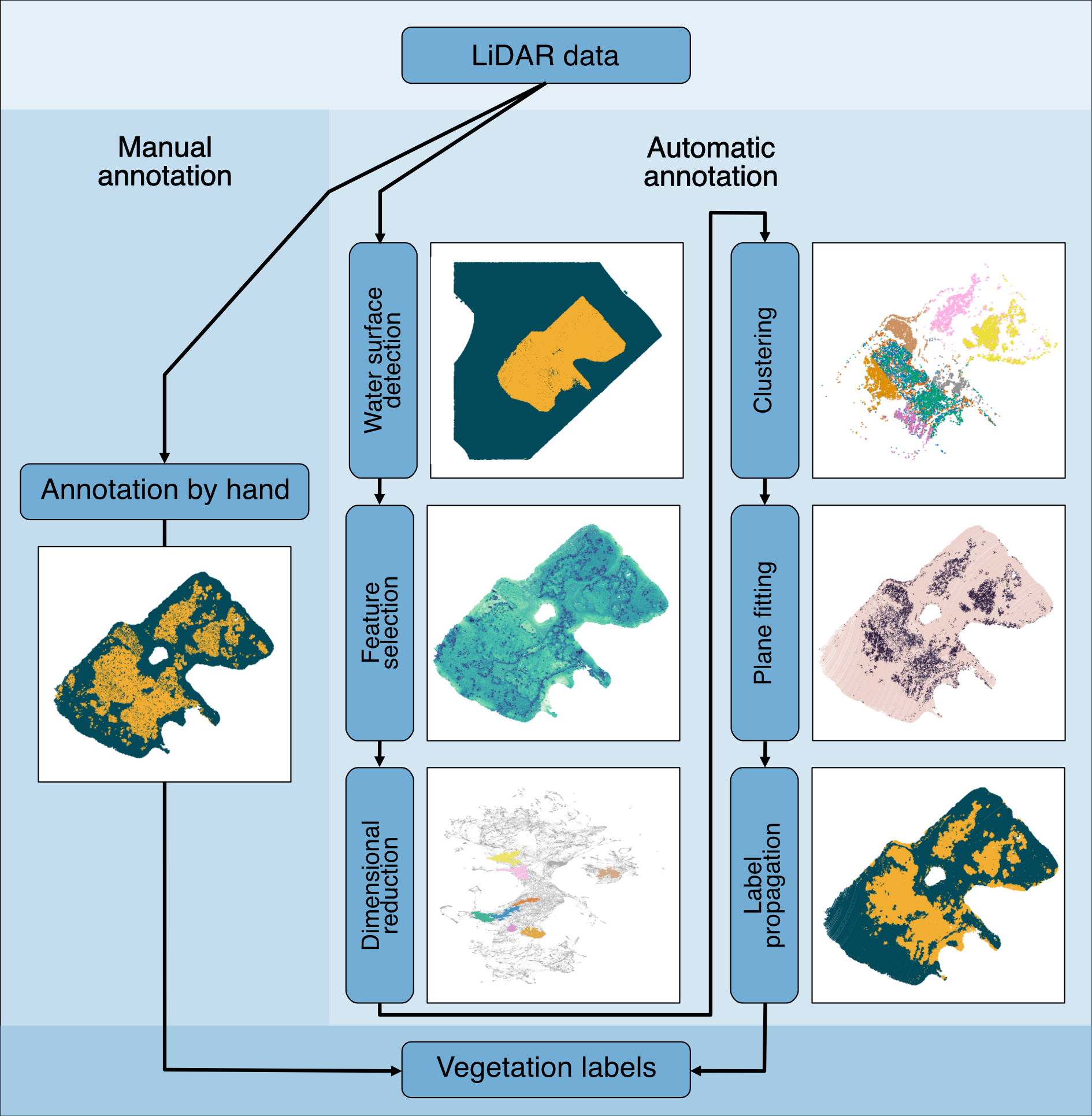
The vegetation classification algorithm is split into three major components, consisting of six steps including the preprocessing (Fig. 4): (i) Feature selection and normalization (Section 3.1–3.5), (ii) Dimensional reduction and clustering (Section 3.6–3.7) and (iii) Vegetation classification with additional label improvement (Section 3.8–3.9). The features obtained from the LiDAR point cloud can be represented as a high-dimensional dataset, which is reduced to a two-dimensional dataset with UMAP. This dimensionally reduced dataset is first clustered, which generates an output of groups which are mostly vegetation. Subsequently, the generated clusters are classified into two categories: vegetation and other, which is achieved through a clusterwise planarity score and further improved by graph theoretical methods, as the clusters do not capture all points belonging to the submerged vegetation.

3.1 LiDAR feature selection

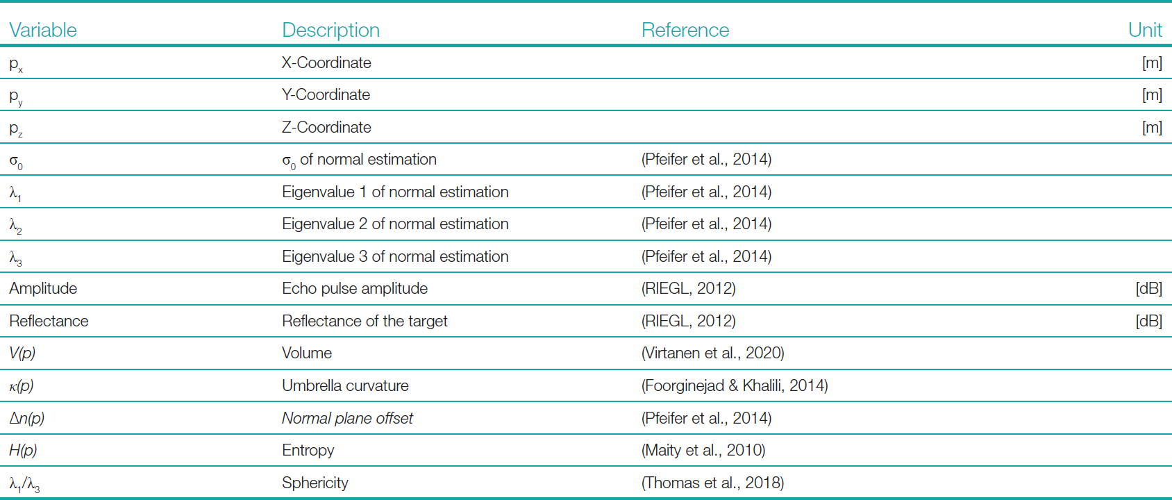
The acquisition of LiDAR data yields a multitude of features for each recorded point, including the coordinates in the selected reference coordinate system, amplitude and reflectance (Pfennigbauer & Ullrich, 2010). Additionally, research-oriented processing of the LiDAR data also makes use of specialized software, such as OPALS (Pfeifer et al., 2014), to calculate normal vectors and eigenvalues. The output of the OPALS software generates values such as σ₀, λ₁, λ₂ and λ₃ (Table 2), generated based on the covariance matrix of the local neighborhood (10 neighbors) within the robust normal estimation (based on the three position vectors), where a robust plane fitting of the selected neighbors is used to calculate the corresponding normal vector (Jutzi & Gross, 2009; Pfeifer et al., 2014; Weinmann et al., 2015). In the same processing step an offset ∆n(p) for the fitted plane of the normal vector is calculated, introducing a local planarity measure (Pfeifer et al., 2014). In addition, we calculate the umbrella curvature and volume of the local neighborhood of each point. For this, we first introduce a clear definition of the neighborhood (Section 3.2) and then calculate the umbrella curvature (Section 3.3) and volume (Section 3.4) for the selected points. Lastly, we calculate two more parameters based on the OPALS processing output: the sphericity and the entropy. Both calculated features provide insight into the object’s structure beyond the single eigenvalue variables and therefore finalize the feature space (Jutzi & Gross, 2009; Thomas et al., 2018). The constructed array of features for each point (Table 1) contains substantial information about all points within the surveyed ecosystem and thus builds the basis for a higher-dimensional analysis. In conclusion, the more independent features describing the object can be extracted, the more stable the association becomes (Thomas et al., 2018).

3.2 Neighborhood and kNN-graph

Before we introduce the umbrella curvature (Section 3.3) and volume (Section 3.4), some preparatory steps are required, as these are measures of local neighborhoods within the point cloud. Let 𝒫 be the set of position vectors from the observation (the set of x-y-z coordinates of the point cloud) for each observation p ∈ 𝒫. We define the local neighborhood by selecting the 10 closest points for each point p ∈ 𝒫 in 3D space, where the initial point p ∈ 𝒫 is counted as the first point of the selected set. As a result, we can define the partially ordered set of all distances from p ∈ 𝒫 as 𝒟(p) and apply this definition to characterize the local neighborhood 𝒩(p) of p ∈ 𝒫 as:

(1)

(2)

In addition, the neighborhood definition allows us to create a network representation of the LiDAR point cloud. For this, we define the k-nearest neighbors graph (kNN-graph) of the point cloud on the basis of the neighborhood 𝒩(p) for all p ∈ 𝒫. The created undirected unweighted graph consists of the subset of all unique edges and all points given by the neighborhood definition. Initially each point has 9 edges to its closest neighbors, but as two points in the local neighborhood are automatically each other’s neighbors, the duplicated edges resulting in those connections are removed to obtain a simple graph. Furthermore, if the surveyed area is sufficiently connected, the graph also consists of a single connected component.

In accordance with current best practices in high-dimensional data analysis, the neighborhood parameter is again set to 10 (Luecken & Theis, 2019). However, this parameter can be adjusted depending on the dataset size, spatial resolution or other factors affecting the extent of the vegetation features that can be detected with the LiDAR system. The advantage of the generated graph representation is shown in Section 3.9. There, the kNN-graph is used to improve the final vegetation labels, and therefore the introduction of the neighborhood concept becomes a vital tool in the analysis of structural features within the point cloud dataset.

3.3 Umbrella curvature

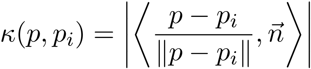
To measure the roughness in the point cloud, we deploy the measure of umbrella curvature in the local neighborhood of each point. The umbrella curvature for a point p ∈ 𝒫 is defined as the sum of the curvatures between the current point p and its n closest neighbors, using the inner product and the normal vector n to the fitted plane at p (Foorginejad & Khalili, 2014).

(3)

Calculating this curvature for each point in the neighborhood, we get the umbrella curvature of p as

(4)

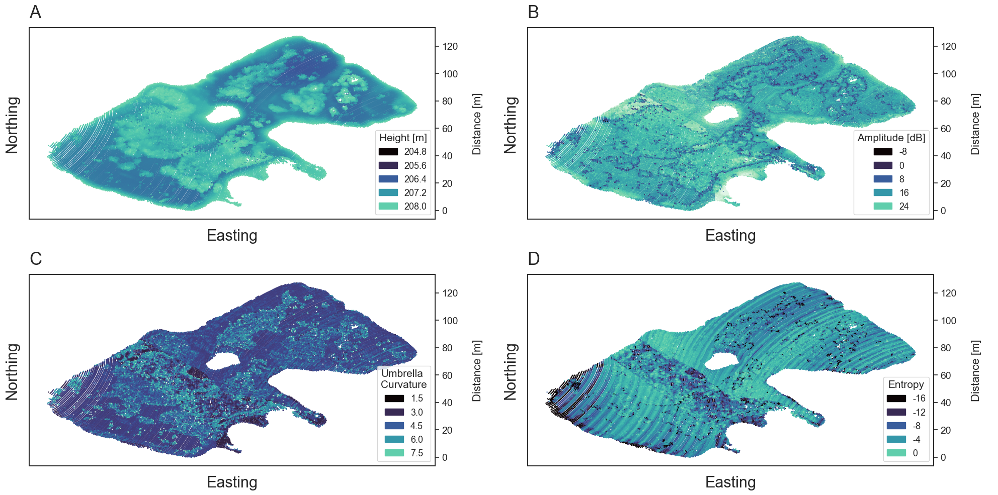
This measure can be compared to the amount an umbrella opens up with p as the umbrella’s center (Foorginejad & Khalili, 2014). In the context of submerged vegetation, this measure indicates whether the neighborhood of a point is smooth or whether it has a varying vertical extent (Fig. 5).

3.4 Volume

To further expand the feature space related to structural features, we add a measure of volume for each local neighborhood. This measure is based on the volume of the convex hull of the points, which by definition is the smallest convex enclosement of the points selected (Moklyachuk, 2021).

Through the triangulation of the convex polytope, the volume V(p) can be numerically calculated, e.g., using SciPy (Virtanen et al., 2020). The convex hull is a measure for the general neighborhood size and also an estimate of the volumetric point density. Therefore, vegetation points should have larger volume as the points within the neighborhood exhibit varying vertical extent due to the fact that the laser pulses are reflected at different heights throughout the vegetation, while the terrain in the pond is generally smooth.

3.5 Entropy

Lastly, we also calculate the entropy H(p) of the scattering object, which relates to the randomness of the scattering target (Maity et al., 2010; Jin & Cloude, 1994). Low entropy values indicate a single dominant scattering element and high values imply that the target has scattering components, where no single component dominates (Maity et al., 2010). The entropy H of the point p and the eigenvalues λ₁, λ₂ and λ₃ can be calculated through

(5)

The introduced parameter improves the understanding of the randomness of the scattered media and therefore further improves the understanding of the measured target (Fig. 5). A higher randomness corresponds to a higher diversity in the spatial distribution of the points, which is associated with vegetation canopy (Liu et al. 2022)

3.6 Data normalization

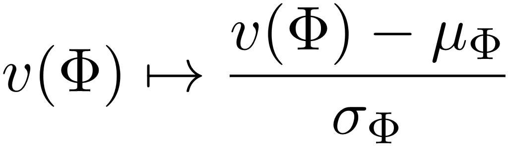
After feature selection, the next step in the analysis is to homogenize the value range of the individual features (z-score transformation), as they have different scales (Sainburg et al., 2021; Pedregosa et al., 2011). Taking all features F as one part of the dimensional input and the number of points in the point cloud as the second, a high-dimensional dataset with dimension of |F| can be constructed. This dataset cannot be visualized in conventional ways, as the data structure now has |𝒫| points along |F| dimensions. In terms of data structure, the new high-dimensional dataset corresponds to a matrix of the shape |𝒫| × |F|. To finalize the data preparation for the dimensional reduction, a standard scaler has to be applied to all feature values (z-score normalization), otherwise the values would form different distributions based on their maximum or mean values rather than displaying similar patterns across all features. Let Φ ∈ F be a feature of the point cloud with feature values v(Φ), mean value µ_Φ and standard deviation σ_Φ, then the standard scaler is given by the following mapping.

(6)

3.7 Dimensional reduction and clustering

All points of the point cloud are now in a form that allows to look for patterns regarding their features. But as these features are given in a high-dimensional space, they are affected by the “curse of high-dimensionality”, meaning that commonly used unsupervised methods create unconventional results depending on the metrics used (Assent, 2012; Beyer et al., 1999). Therefore, we deploy a technique often used in single-cell clustering (Luecken & Theis, 2019), where we use dimensional reduction techniques to project the feature space to a regular two-dimensional space, using UMAP (Sainburg et al., 2021). This dimensional reduction method approximates the high-dimensional shape of the data and creates a two-dimensional image of the underlying manifold through mathematical processing (Sainburg et al., 2021). This is comparable to a workflow based on PCA, with the additional advantage of capturing the shape of the high-dimensional dataset and translating high-dimensional similarity of features to a two-dimensional spatial proximity, which can be detected using clustering methods (Kurita, 2019).

To separate the dimensional reduction into groups of interest, clustering is applied to the created dimensionally reduced dataset. To group the points into clusters of interest and remove outliers, a density-based clustering algorithm (DBSCAN) is applied to the dimensionally reduced dataset (Pedregosa et al., 2011; Schubert et al., 2017; Ester et al., 1996). DBSCAN strongly depends on the selection of the epsilon parameter, which defines the maximum distance between two samples to be considered in the neighborhood of one other (Pedregosa et al., 2011). This in turn influences the size and furthermore the number of clusters. For the vegetation classification, epsilon is fine-tuned within a range of 0.04 to 0.06, which corresponds to a sufficiently small neighborhood in the dimensionally reduced dataset. The epsilon parameter is selected within this range, to avoid over-clustering the data and simultaneously extract more than a single cluster. By applying DBSCAN, the different clusters of similar features can be extracted, which then form the basis for the following vegetation annotation. The extracted clusters are furthermore filtered in size by a general minimum cluster size of 500 points, as the vegetation should contain a large number of points and this helps to avoid excessive clustering of the data. The identified clusters can now be backtracked into the original LiDAR point cloud leaving multiple groupings of points with similar features, which are rooted in higher dimensional similarity rather than close spatial proximity. These clusters, extracted from the dimensionally reduced dataset, represent an initial extraction of the geometric similarities, displayed by the vegetation. Therefore, the groups detected by DBSCAN can be seen as the initial classification of submerged vegetation, with a subset of terrain that displays similar feature characteristics.

3.8 Vegetation classification via plane fitting

For each cluster that is not removed due to the minimum point filtering or DBSCAN outlier detection, a plane is based on the x-y-z-vector positions of the points and the distance to the plane is calculated for each point of the cluster, as this improves the vegetation within the clustering by removing planar clusters (terrain). Vegetation generally results in uneven surfaces with high vertical differences of the points due to multiple reflections in different height levels, recorded by the LiDAR system. In contrast, the underwater terrain of the surveyed ponds is generally smooth. Additionally, with the medium sized footprint of the deployed LiDAR system, small deviations in height are smoothed out. Therefore, the plane fitting creates two groups of clusters on a macro scale (compared Section 3.1), with either small or large pointwise deviations from the plane. To classify the vegetation, we introduce here a filtration of the plane fitting residual, where points with above mean residual are classified as vegetation and those below as terrain.

3.9 Label propagation

The vegetation detection method has so far introduced an initial classification based on UMAP, clustering and plane fitting. However, this classification is sparse, as the clustering fails to extract all vegetation points and therefore does not sufficiently capture the vegetation within the submerged ecosystem. We therefore improve the existing labels through label propagation, a tool commonly deployed in graph theory (Raghavan et al., 2007). For the label propagation, the neighborhood in the form of the kNN-graph introduced in the Section 3.2 is used. The labels from the initial classification are transferred to the vertices of the kNN-graph and the method then compares the labels of neighboring vertices, updating the vertex label based on a majority of labels within the current neighborhood (Csardi & Nepusz, 2006). By only adjusting the terrain labels and keeping all initial vegetation labels, the label propagation can extend the vegetation labels to vertices in the neighborhood that feature a high connectivity to vertices with the same label. Through this extension of the vegetation labels, the general under-performance of the UMAP extraction can be compensated and thus denser vegetation clusters can be annotated.

3.10 Macrophyte canopy height estimation

Based on the aquatic vegetation extracted from the dataset, a map of the vegetation height can be created. This canopy height estimation uses the points classified as vegetation to estimate the height in relation to a digital terrain model (DTM) generated from the points classified as underwater terrain. To construct the DTM, we use the point cloud processing software CloudCompare (CloudCompare 2.12.4, 2024), which features a rasterization tool to generate DTMs. There the DTM is based on the shoalest z-values of the non-vegetation points for each grid cell, accounting for potential outliers in the water column. Furthermore, the z-values are computed based on a grid distance of 2.5 m. To derive the macrophyte canopy height above the interpolated ground, we can now subtract the height of each vegetation point from the closest DTM ground point and record all positive differences for the canopy height. The height estimation based on the averaged z-values, holds true for the surveyed ponds, as the vegetation within the pond predominantly consists of Charophyceae. This type of vegetation grows as a dense population and thus the majority of laser pulses are being reflected by the canopy. This generates a generally uniform point cloud, representing the uppermost layer of the vegetation as only few LiDAR echo pulses of the stem are recorded.

3.11 Area and volume estimation of the macrophyte population

The area of the ponds covered with submerged vegetation can be estimated by rasterizing both the water surface area and the submerged vegetation and comparing the created cells. This is done by first rasterizing the pond into 1m 𝗑 1m cells, both for the clustered vegetation 𝒞(P_V) and the pond’s water surface 𝒞(P_W). For this, let 𝒫_V be the set of points classified as vegetation and 𝒫_W be the set of water surface points extracted with the SVB method (Schwarz et al., 2019). This approximation of the water surface could further be enhanced by manual annotation, but to improve on the automated detection, the provided surface model is solely based on the SVB algorithm. Therefore an underestimation of the water surface has to be taken into account, which typically only affects the closest . The cells are calculated by rounding the x- and y-coordinates of the vegetation and the water surface to the nearest integer and merging all cells with the same rounded coordinates. Dividing the vegetated area by the water surface area then provides an estimation of the vegetation coverage A(𝒫_V) [%] of the pond.

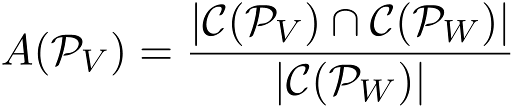(7)

Furthermore, by multiplying the area of the vegetation cell c_i ∈ 𝒞(𝒫_V) with the average vegetation height of the cell h_mean(c_i), a cell-wise vegetation volume can be calculated. by summing up all cell volumes, an overall estimation of the vegetation volume of the pond 𝒱(P_V) [m³] can be derived, based on the canopy type and canopy height estimation (Section 3.10).

(8)

4 Results

To establish the context for the subsequent discussion, the results presented in this section display the labels produced by the classifier, a visual comparison using orthophotos and an overall quantitative evaluation. This provides an extensive insight into the labels produced by the classification, as well as a quantitative evaluation approach.

4.1 Vegetation classification

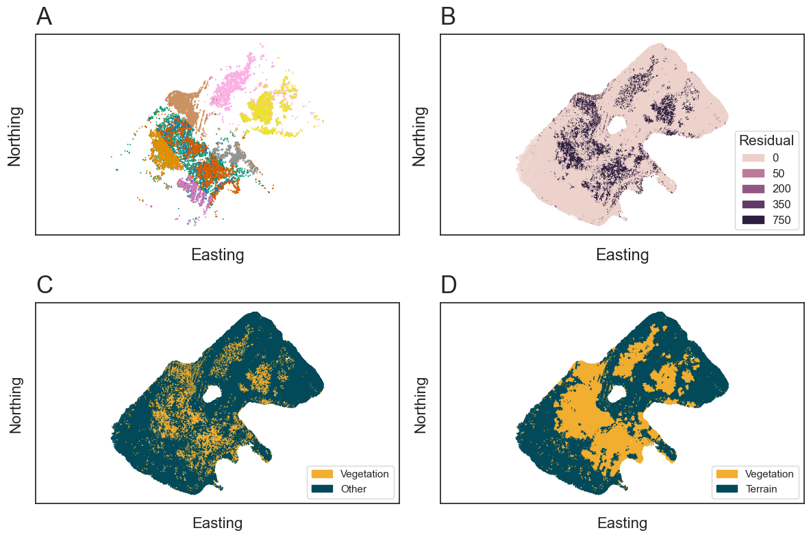
The results of the introduced vegetation classification can be seen in Fig. 6, where each major step of Section 3 is shown for Pond 2. After the preprocessing (Section 2.3) and the feature selection (Section 3.1–3.5), the vegetation classifier normalizes the data and extracts clusters of potential vegetation through dimensional reduction (Sections 3.6 and 3.7). The extracted clusters can be seen in Fig. 6a, where each cluster is larger than the minimum of 500 points and consists of points sharing a similarity of features. For each cluster, the plane fitting is applied (Section 3.8), distinctly separating the clusters into two groups of high and low plane fitting residuals (Fig. 6b). The high residual clusters are classified as vegetation and create an initial sparse classification (Fig. 6c), which is improved by the label propagation (Section 3.9). Leading to the final vegetation classification of the point cloud displayed in Fig. 6d.

4.2 Visual comparison to photogrammetric data

The orthophotos allow for a visual comparison between the generated labels and the vegetation visible in the two ponds. In both cases, the classified LiDAR vegetation points can be compared with the vegetation visible in the ortho images (Fig. 7).

4.3 Comparison of manual annotations

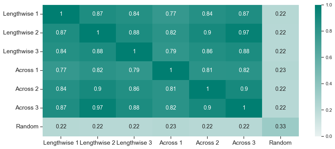
For the manual annotation of the dataset, three experts in the field of bathymetry were selected. To evaluate labeling biases and put the results of Section 4.4 into a more comparative context, the individual manual annotations are cross-validated and furthermore compared to a randomly shuffled array of vegetation and terrain labels (Fig. 8). The results from Fig. 8 highlight the subjectivity of annotating point cloud data and the difference depending on the field of view from which the data is annotated. In addition, the distinction between true vegetation echoes and echoes from volume backscattering in the water column represents a general challenge for research in the extraction of underwater LiDAR echoes (Li et al., 2024). Therefore, the comparison underlines the minimum and maximum possible scores for the vegetation clustering.

4.4 Accuracy assessment with annotated data

To evaluate the vegetation detection method on a quantitative basis, we compare the generated labels to manually annotated labels for the same pond. This is done for several metrics, displayed in Table 2. Each score compares the annotated vegetation labels to the labels of the classification algorithm and outputs a score between 0 and 1. The lowest possible score is 0, indicating a bad fit, and 1 indicates an ideal consensus between the two sets of labels (Pedregosa et al., 2011).

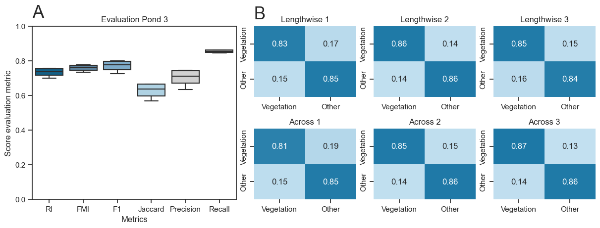
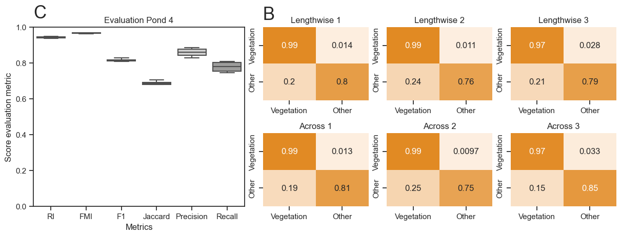
With the dataset introduced in Section 2.2 we can evaluate the labels generated by the described vegetation classification method. The quantitative results are reported in Fig. 9 displaying the confusion matrix of each manual annotation compared to the automatically generated labels. The matrices furthermore indicate the type I errors (false positives) and type II errors (false negatives) of the classification, which fall within a 10–30 % margin. Similarly, the true positives are approximately 80 % to 99 %. The results for Pond 3a display a true positive rate of close to 100 %, while for Pond 2 the scores reach a maximum of 87 %. Contrary, the true negatives are lower for Pond 2 compared to Pond 3a. This indicates that the method overestimated the vegetation in Pond 2, while in Pond 3a the vegetation was underestimated.

The applied metrics (RI, FMI, F1, Jaccard, Precision, Recall) are commonly used for assessing clustering methods, especially for two-class problems as in our case (Amigo et al., 2009; Fahad et al., 2014; Pedregosa et al., 2011). Most of the evaluation metric scores are in the range from 0.54 to 0.96 (Figs. 9a and 9c). For the majority of the scores (all except Jaccard), the scores are based on a comparison between true positives and true negatives and false positives and false negatives. Therefore, a score close to 1 reflects high true positives and true negatives, with furthermore low type I and II errors. The Jaccard index in contrast is based on set intersection, a score of 1 indicating that the labels share the exact same points. Comparing the different metrics therefore outlines how high the type I and II errors are for each pond and furthermore how identical the sets of labels are. In Pond 2, this mathematical basis of the metrics is reflected in a lower overall score due to the presence of higher errors. Contrary, Pond 3a, which exhibits more distinct vegetation, has an increased score.

We can conclude that the performance of the vegetation classification for Pond 2 and Pond 3a stands between 0.74 and 0.84 mean performance, across all metrics. Pond 3a has an increased score due to higher true positives and true negatives, compared to Pond 2.

4.5 Vegetation parameters

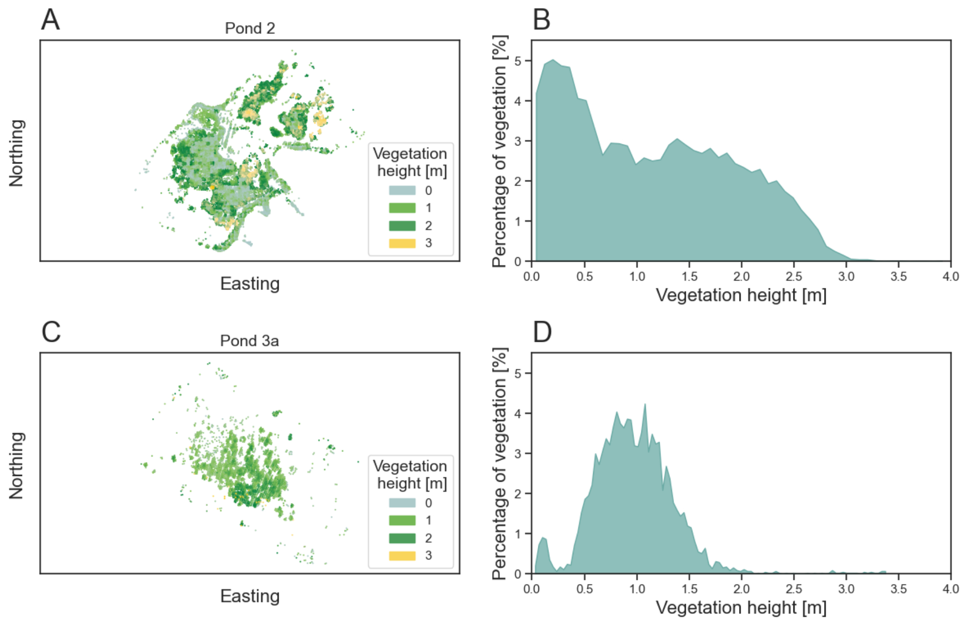
The vegetation parameters obtained through the methodology, outlined in Section 3.10, can be expressed as a map of the canopy height (Figs. 10a and 10c) and distribution plots (Figs. 10d and 10b). For the calculated parameters of the Section 3.11 the results for the ponds are shown in Table 3.

The vegetation height map (Fig. 10) highlights the differences in vegetation growth for both ponds. The complex structures visible in Pond 2 show varying vertical extent. Patches of larger vertical extent are mostly concentrated in dense regions with small spatial extent and regions of low grown vegetation span across larger areas of the pond. Pond 3a, in turn, has a limited macrophyte population with a single patch of notable vegetation. These differences are furthermore reflected in the quantitative parameters of both ponds displayed in Table 3. Additionally, the differences in vertical extent can be seen in the two distributions displayed in Figs. 10b and 10d. There, Pond 2 displays a wide range of different heights with a higher degree of low vegetation (<0.5 m) compared to high vegetation (0.5–3 m), while Pond 3a displays a distribution of similar vertical extent.

5 Discussion

5.1 Challenges through scan strip overlap

One of the challenges in the dataset of Pond 2 is that the dataset contains points from two partially overlapping flight strips, requiring downsampling to achieve a homogeneous point density, which is a prerequisite for the introduced method. A disadvantage of the selected approach is that through the cutoff, the distribution of the point cloud changes and thus a partial bias towards the overlap remains. This change in point distribution is clearly visible in Fig. 5d and can also be detected in Fig. 6a. In Fig. 6a, the change in structure can be seen in the green and orange cluster. There, the clusters from the same outlines as seen in Fig. 5d highlight the similarity within the strip overlap and furthermore in the high-dimensional feature space.

The artificially increased similarity of the strip overlap could potentially be overcome by the selection of a fixed distance neighborhood instead of a k-nearest neighborhood and should improve deviations of the eigenvalue related measures, as the neighborhood selection is influenced by the point density. Therefore, the vegetation classification method underperforms in the case of Pond 2, which suggests using a more homogeneous thinning approach to avoid bias in the strip overlap.

Other factors to consider are the alignment of the point clouds. In case of Pond 2, the two point clouds were not perfectly aligned, leading to discrepancies in the point cloud features. Such offsets of the two flight strips could lead to misaligned terrain points, which could be interpreted by the method as low-grown vegetation. This could be improved through better georeferencing and should ideally minimize distribution-based errors (Pöppl et al., 2024). Overall, the observations from the dataset suggest the importance of ensuring the highest possible quality of alignment through pre-processing of the LiDAR data and to correct remaining feature offsets based on differences in densities to overcome potential offsets.

5.2 Parameter selection and supervision

A common challenge in high-dimensional data analysis, in addition to dimension reduction, is the extraction of features from the projected space (Luecken & Theis, 2019; Allaoui et al., 2020). In a two- or three-dimensional projection of the data, the distances do not relate to physical based metrics, which can induce problems in the parameter selection of clustering algorithms. Therefore, the selection of the correct clustering algorithm combined with a good parameter selection is essential for extracting good results from the dimensionally reduced datasets. For many of the commonly used clustering methods for two-dimensional projection of the data, a supervision or revisiting of the clustering step is required. This often results in fine-tuning distance parameters or clustering centroids (Luecken & Theis, 2019). Other algorithms use graph-based methods or multi-resolution clustering to reduce human supervision and time spent on parameter fine-tuning (Luecken & Theis, 2019; Levine et al., 2015; Wolf et al., 2019; Zappia & Oshlack, 2018). These methods show promising results in other fields, but require more complex workflows or, in the case of graph-based methods, data with more dimensions than the LiDAR dataset provides (MacQueen et al., 1967; Levine et al., 2015; Wolf et al., 2019).

Therefore, we use a simpler approach in this paper based on commonly used density-based clustering (DBSCAN), which further provides an integrated outlier detection (Pedregosa et al., 2011; Schubert et al., 2017; Ester et al., 1996). The downside of this method is the necessity of a resolution parameter for the dimensionally reduced space. DBSCAN uses a Euclidean distance measure to extract the clusters, which, if run with standard parameters, might lead to an over- or under-clustering of the projection space. This parameter requires supervision and a general knowledge of the dispersion of vegetation in the lake to achieve maximum accuracy. A promising solution for the extraction of detailed clusters without over-clustering is the emerging multi-resolution consensus clustering approach (Goggin & Zunder, 2023). This would cluster at different resolutions and merge clusters based on similarity, making the parameter selection obsolete (Goggin & Zunder, 2023; Zappia & Oshlack, 2018).

5.3 Annotation in submerged datasets

A different source of uncertainty is the lack of objective and reliable ground truth data. The general approach of labeling data is by human annotation and comparison of the labels to the method’s output. The challenge in manual annotation is that in regions of ambiguous groupings, the annotations are different due to subjective assessments, which is why the labels must not only be compared to the generated labels by the method, but also among each other (Zhu et al., 2019). This creates the opportunity to give an evaluation range for the labeled data. In general, the evaluation of point cloud data profits from cross-comparison, as the large volume of data and the general complexity of 3D point clouds lead to differences in manual labeling by human operators (Anand & Rajalakshmi, 2023; Ye et al., 2021). It is furthermore noted that aerial images could potentially further be used for scene reconstruction via Dense Image Matching (Mandlburger, 2019). Such a comparison is currently outside the scope of this study, as the resolution and quality of the images are sub-optimal. Nonetheless, future studies could use high resolution images to reconstruct the vegetation canopy and through the comparison of the data, could potentially improve the evaluation.

5.4 Ecological insights

The extraction of the surface area covered with submerged vegetation and the vegetation volume both are quantities of importance in the analysis of the aquatic ecosystem. These measurements are already common for forestry LiDAR data (Zhou et al., 2022) and are important to the monitoring of ecosystems. The area and volume of the vegetation are used to estimate the biomass in the surveyed area and monitor vital changes of the ecosystem (Michalowska & Rapiński, 2021; Kumpumäki et al., 2015). Due to the larger footprint (0.91 m diameter) of the LiDAR system used in the survey, the measures introduced in this survey are based on large cells (1 m²) and thus do only represent rough estimates of the vegetation parameters. This could potentially be improved by using UAV-borne surveys or smaller beam divergences for classical data acquisition with crewed aircraft, as this would allow for a higher point density and a higher spatial resolution, making smaller cells possible. In conclusion, the area and volume estimation techniques introduced in this study do not require expensive in-situ measurements and are solely data driven. This improves bottlenecks in the analysis of vast regions of aquatic landscapes, but could benefit from higher spatial resolutions.

6 Conclusion

The introduced vegetation detection method benefits from recent advancements in high-dimensional data analysis and establishes an automated workflow for vegetation detection with minimal parameter selection. Through the extension of standard LiDAR features in addition with calculated structural descriptors, a high-dimensional dataset of the LiDAR point cloud can be obtained. This high-dimensional dataset can then be analyzed for similarities of features through dimensional reduction and clustering. Each detected cluster is further tested for planarity to extract the clusters representing vegetation, which (i) builds the basis for vegetation labeling of the point cloud with only minimal parameter tuning and (ii) furthermore allows for estimation of vegetation area and volume.

This enables ecological analysis of submerged ecosystems, which is beneficial in a broader context as obtaining fundamental insights into the working principles and changes of aquatic ecosystems have become a primary focus of climate monitoring. Overall, the introduction of bathymetric LiDAR shows promising results for the automated extraction of vegetation in LiDAR point cloud and enables future work to go beyond what is currently possible using only in-situ measurements.

References

Ackleson, S. and Klemas, V. (1987). Remote sensing of submerged aquatic vegetation in lower Chesapeake Bay: A comparison of landsat MSS to TM imagery. Remote Sensing of Environment, 22(2), pp. 235–248.

Aleksandra, K., Fantina, M., Marco, S., Ferrarin, C. and Giacomo, M. G. (2015). Assessment of submerged aquatic vegetation abundance using multibeam sonar in very shallow and dynamic environment. The Lagoon of Venice (Italy) case study. In 2015 IEEE/OES Acoustics in Underwater Geosciences Symposium (RIO Acoustics), pp. 1–7. IEEE.

Allaoui, M., Kherfi, M. L. and Cheriet, A. (2020). Considerably Improving Clustering Algorithms Using UMAP Dimensionality Reduction Technique: A Comparative Study, International conference on image and signal processing, pp. 317–325. Springer International Publishing.

Amani, M. and Mahdavi, G. (2021). ML and LiDAR to map aquatic vegetation.

Amigo, E., Gonzalo, J., Artiles, J. and Verdejo, F. (2009). A comparison of extrinsic clustering evaluation metrics based on formal constraints. Information retrieval, 12, pp. 461–486.

Anand, B. and Rajalakshmi, P. (2023). Pipeline for automation of lidar data annotation. In 2023 IEEE Sensors Applications Symposium (SAS), pp. 1–6. IEEE.

Assent, I. (2012). Clustering high dimensional data. WIREs Data Mining and Knowledge Discovery, 2(4), pp. 340– 350.

Bellman, R. and Kalaba, R. (1959). A mathematical theory of adaptive control processes. Proceedings of the National Academy of Sciences, 45(8), pp. 1288-1290.

Beyer, K., Goldstein, J., Ramakrishnan, R. and Shaft, U. (1999). When is “nearest neighbor” meaningful? In Database Theory—ICDT99: 7th International Conference Jerusalem, Israel, January 10–12, 1999 Proceedings 7, pp. 217–235. Springer.

Blondel, P. (2008). A review of acoustic techniques for habitat mapping. Hydroacoustics, 11, pp. 29–38.

Calantropio, A., Menna, F., Skarlatos, D., Balletti, C., Mandlburger, G., Agrafiotis, P., Chiabrando, F., Lingua, A. M., Giaquinto, A. and Nocerino, E. (2024). Under and through water datasets for geospatial studies: the 2023 ISPRS scientific initiative “nautilus”. ISPRS Annals of the Photogrammetry, Remote Sensing and Spatial Information Sciences, 10, pp. 33–40.

Carpenter, S. R. and Lodge, D. M. (1986). Effects of submersed macrophytes on ecosystem processes. Aquatic Botany, 26, pp. 341–370.

Chen, L. (2009). Curse of Dimensionality. In L. Liu and M. T. Özsu (Eds.), Encyclopedia of Database Systems. Springer, Boston, MA. https://doi.org/10.1007/978-0-387-39940-9_133

CloudCompare (2024). 3D point cloud and mesh processing software. Open source project, GPL.

Coops, H., Kerkum, F. C. M., van den Berg, M. S. and van Splunder, I. (2007). Submerged macrophyte vegetation and the european water framework directive: assessment of status and trends in shallow, alkaline lakes in the netherlands. Hydrobiologia, 584(1), pp. 395–402.

Csardi, G. and Nepusz, T. (2006). The igraph software. Complex syst, 1695, pp. 1–9.

De Grandpre, A., Kinnard, C. and Bertolo, A. (2022). Open-source analysis of submerged aquatic vegetation cover in complex waters using high-resolution satellite remote sensing: An adaptable framework. Remote Sensing, 14(2), p. 267.

Dierssen, H. M., Ackleson, S. G., Joyce, K. E., Hestir, E. L., Castagna, A., Lavender, S. and McManus, M. A. (2021). Living up to the hype of hyperspectral aquatic remote sensing: Science, resources and outlook. Frontiers in Environmental Science, 9.

Domingos, P. (2012). A few useful things to know about machine learning. Communications of the ACM, 55(10), pp. 78–87.

Espel, D., Courty, S., Auda, Y., Sheeren, D. and Elger, A. (2020). Submerged macrophyte assessment in rivers: An automatic mapping method using pleiades imagery. Water Research, 186, 116353.

Ester, M., Kriegel, H.-P., Sander, J., Xu, X., et al. (1996). A density-based algorithm for discovering clusters in large spatial databases with noise. KDD, 96, pp. 226–231.

Fahad, A., Alshatri, N., Tari, Z., Alamri, A., Khalil, I., Zomaya, A. Y., Foufou, S. and Bouras, A. (2014). A survey of clustering algorithms for big data: Taxonomy and empirical analysis. IEEE transactions on emerging topics in computing, 2(3), pp. 267–279.

Federal Office of Metrology and Surveying, BEV, (2024). Austrian map online. https://www.bev.gv.at/Services/Produkte/Austrian-Map/Austrian-Map-online.html (accessed 10 November 2024).

Foorginejad, A. and Khalili, K. (2014). Umbrella curvature: A new curvature estimation method for point clouds. Procedia Technology, 12, pp. 347–352.

García-Gutiérrez, J., Martínez-Álvarez, F., Troncoso, A. and Riquelme, J. C. (2015). A comparison of machine learning regression techniques for LiDAR-derived estimation of forest variables. Neurocomputing, 167, pp. 24–31.

Goggin, S. M. and Zunder, E. R. (2023). A hyperparameter-randomized ensemble approach for robust clustering across diverse datasets.

Held, P. and Schneider von Deimling, J. (2019). New feature classes for acoustic habitat mapping—a multibeam echosounder point cloud analysis for mapping submerged aquatic vegetation (sav). Geosciences, 9(5), p. 235.

Jin, Y.-Q. and Cloude, S. R. (1994). Numerical eigenanalysis of the coherency matrix for a layer of random nonspherical scatterers. IEEE Transactions on Geoscience and Remote Sensing, 32(6), pp. 1179–1185.

Jutzi, B. and Gross, H. (2009). Nearest neighbour classification on laser point clouds to gain object structures from buildings. The International Archives of the Photogrammetry, Remote Sensing and Spatial Information Sciences, 38(1), pp. 4–7.

Koma, Z., Zlinszky, A., Bekö, L., Burai, P., Seijmonsbergen, A. C. and Kissling, W. D. (2021). Quantifying 3d vegetation structure in wetlands using differently measured airborne laser scanning data. Ecological Indicators, 127, 107752.

Kumpumäki, T., Ruusuvuori, P., Kangasniemi, V. and Lipping, T. (2015). Data-driven approach to benthic cover type classification using bathymetric lidar waveform analysis. Remote Sensing, 7(10), pp. 13390–13409.

Kurita, T. (2019). Principal component analysis (PCA). Computer vision: a reference guide, pp. 1–4.

Levine, J., Simonds, E., Bendall, S., Davis, K., Amir, E.-a., Tadmor, M., Litvin, O., Fienberg, H., Jager, A., Zunder, E., Finck, R., Gedman, A., Radtke, I., Downing, J., Pe’er, D. and Nolan, G. (2015). Data-driven phenotypic dissection of AML reveals progenitor-like cells that correlate with prognosis. Cell, 162(1), pp. 184–197.

Li, N., Truong, M.-L., Schwarz, R., Pfennigbauer, M. and Ullrich, A. (2024). Deep learning assisted exponential waveform decomposition for bathymetric lidar. The International Archives of the Photogrammetry, Remote Sensing and Spatial Information Sciences, XLVIII-2-2024, pp. 195–202.

Liu, X., Ma, Q., Wu, X., Hu, T., Liu, Z., Liu, L., Guo Q. & Su, Y. (2022). A novel entropy-based method to quantify forest canopy structural complexity from multiplatform lidar point clouds. Remote Sensing of Environment, 282, 113280.

Lønborg, C., Thomasberger, A., Stæhr, P. A. U., Stockmarr, A., Sengupta, S., Rasmussen, M. L., Nielsen, L. T., Hansen, L. B. and Timmermann, K. (2021). Submerged aquatic vegetation: Overview of monitoring techniques used for the identification and determination of spatial distribution in European coastal waters. Integrated Environmental Assessment and Management, 18(4), pp. 892–908.

Luecken, M. D. and Theis, F. J. (2019). Current best practices in single-cell rna-seq analysis: a tutorial. Molecular Systems Biology, 15(6).

Luo, J., Li, X., Ma, R., Li, F., Duan, H., Hu, W., Qin, B. and Huang, W. (2016). Applying remote sensing techniques to monitoring seasonal and interannual changes of aquatic vegetation in taihu lake, china. Ecological Indicators, 60, pp. 503–513.

MacQueen, J. et al. (1967). Some methods for classification and analysis of multivariate observations. In Proceedings of the fifth Berkeley symposium on mathematical statistics and probability, 1, pp. 281–297. Oakland, CA, USA.

Maity, S., Patnaik, C., Parihar, J. S., Panigrahy, S. and Reddy, K. A. (2010). Study of physical phenomena of vegetation using polarimetric scattering indices and entropy. IEEE Journal of Selected Topics in Applied Earth Observations and Remote Sensing, 4(2), pp. 432–438.

Mandlburger, G. (2019). Through-water dense image matching for shallow water bathymetry. Photogrammetric Engineering amp; Remote Sensing, 85(6), pp. 445–455.

Mandlburger, G. (2022). A review of active and passive optical methods in hydrography. The International Hydrographic Review, 28, pp. 8–52. https://doi.org/10.58440/ihr-28-a15

Mandlburger, G., Kölle, M., Pöppl, F. and Cramer, M. (2023a). Evaluation of consumer-grade and survey- grade uav-lidar. The International Archives of the Photogrammetry, Remote Sensing and Spatial Information Sciences, 48, pp. 99–106.

Mandlburger, G., Pfennigbauer, M., Schwarz, R. and Pöppl, F. (2023b). A decade of progress in topo- bathymetric laser scanning exemplified by the Pielach river dataset. ISPRS Annals of the Photogrammetry, Remote Sensing and Spatial Information Sciences, 10, pp. 1123–1130.

Mandlburger, G., Pfennigbauer, M., Schwarz, R., Flöry, S. and Nussbaumer, L. (2020). Concept and performance evaluation of a novel UAV-borne topo-bathymetric LiDAR sensor. Remote Sensing, 12(6), p. 986.

McCarthy, E. (1997). Acoustic characterization of submerged aquatic vegetation.

Michałowska, M. and Rapiński, J. (2021). A review of tree species classification based on airborne lidar data and applied classifiers. Remote Sensing, 13(3), p. 353.

Moklyachuk, M. (2021). Convex optimization: Introductory course.

Mumby, P. J., Green, E. P., Edwards, A. J. and Clark, C. D. (1999). The cost-effectiveness of remote sensing for tropical coastal resources assessment and management. Journal of Environmental Management, 55(3), pp. 157-166.

Murphy, F., Schmieder, K., Baastrup-Spohr, L., Pedersen, O. and Sand-Jensen, K. (2018). Five decades of dramatic changes in submerged vegetation in lake constance. Aquatic Botany, 144, pp. 31–37.

Nelson, S. A., Cheruvelil, K. S. and Soranno, P. A. (2006). Satellite remote sensing of freshwater macrophytes and the influence of water clarity. Aquatic Botany, 85(4), pp. 289–298.

O’Neill, J. D. and Costa, M. (2013). Mapping eelgrass (zostera marina) in the gulf islands national park reserve of canada using high spatial resolution satellite and airborne imagery. Remote Sensing of Environment, 133, pp. 152–167.

Pedregosa, F., Varoquaux, G., Gramfort, A., Michel, V., Thirion, B., Grisel, O., Blondel, M., Prettenhofer, P., Weiss, R., Dubourg, V., Vanderplas, J., Passos, A., Cournapeau, D., Brucher, M., Perrot, M. and Duchesnay, E. (2011). Scikit-learn: Machine learning in Python. Journal of Machine Learning Research, 12, pp. 2825–2830.

Pfeifer, N., Mandlburger, G., Otepka, J. and Karel, W. (2014). OPALS – a framework for airborne laser scanning data analysis. Computers, Environment and Urban Systems, 45, pp. 125–136.

Pfennigbauer, M. and Ullrich, A. (2010). Improving quality of laser scanning data acquisition through calibrated amplitude and pulse deviation measurement. In M. D. Turner and G. W. Kamerman (Eds.), SPIE Proceedings. SPIE.

Pöppl, F., Ullrich, A., Mandlburger, G. and Pfeifer, N. (2024). A flexible trajectory estimation methodology for kinematic laser scanning. ISPRS Journal of Photogrammetry and Remote Sensing, 215, pp. 62–79.

Preston, J. (2009). Automated acoustic seabed classification of multibeam images of Stanton Banks. Applied Acoustics, 70(10), pp. 1277–1287.

Raghavan, U. N., Albert, R. and Kumara, S. (2007). Near linear time algorithm to detect community structures in large-scale networks.

RIEGL (2012). LAS extrabytes implementation in RIEGL software. Whitepaper, p. 12.

RIEGL (2023). Datasheet RIEGL VQ-840-G.

Rowan, G. S. L. and Kalacska, M. (2021). A review of remote sensing of submerged aquatic vegetation for non-specialists. Remote Sensing, 13(4), p. 623.

Sabol, B. M., Eddie Melton, R., Chamberlain, R., Doering, P. and Haunert, K. (2002). Evaluation of a digital echo sounder system for detection of submersed aquatic vegetation. Estuaries, 25(1), pp. 133–141.

Sainburg, T., McInnes, L. and Gentner, T. Q. (2021). Parametric UMAP Embeddings for Representation and Semisupervised Learning. Neural Computation, 33(11), pp. 2881–2907.

Saputra, L. R. and Radjawane, I. M. (2022). Seabed coverage classification using lidar bathymetry.

Schiagintweit, G. E. O. (1993, October). Real-time acoustic bottom classification for hydrography a field evaluation of RoxAnn. In Proceedings of OCEANS’93, pp. III-214. IEEE.

Schmieder, K. (1995). Submersed macrophytes of two habitats in lake constance (untersee) and their relations to chemical composition of surface and sediment interstitial water. Acta Botanica Gallica, 142(6), pp. 651–657.

Schmieder, K. (2004). European lake shores in danger—concepts for a sustainable development. Limnologica, 34(1–2), p. 3–14.

Schubert, E., Sander, J., Ester, M., Kriegel, H. P. and Xu, X. (2017). Dbscan revisited, revisited: Why and how you should (still) use DBSCAN. ACM Transactions on Database Systems, 42(3), pp. 1–21.

Schwarz, R., Mandlburger, G., Pfennigbauer, M. and Pfeifer, N. (2019). Design and evaluation of a full-wave surface and bottom-detection algorithm for lidar bathymetry of very shallow waters. ISPRS Journal of Photogrammetry and Remote Sensing, 150, pp. 1–10.

Schwarz, R., Pfeifer, N., Pfennigbauer, M. and Ullrich, A. (2017). Exponential decomposition with implicit deconvolution of lidar backscatter from the water column. PFG – Journal of Photogrammetry, Remote Sensing and Geoinformation Science, 85(3), pp. 159–167.

Serpetti, N., Heath, M., Armstrong, E. and Witte, U. (2011). Blending single beam RoxAnn and multi-beam swath QTC hydro-acoustic discrimination techniques for the Stonehaven area, Scotland, UK. Journal of Sea Research, 65(4), pp. 442–455.

Shi, S., Bi, S., Gong, W., Chen, B., Chen, B., Tang, X., Qu, F. and Song, S. (2021). Land cover classification with multispectral LiDAR based on multi-scale spatial and spectral feature selection. Remote Sensing, 13(20), p. 4118.

Thomas, H., Deschaud, J.-E., Marcotegui, B., Goulette, F. and Gall, Y. L. (2018). Semantic classification of 3d point clouds with multiscale spherical neighborhoods.

Virtanen, P., Gommers, R., Oliphant, T. E., Haberland, M., Reddy, T., Cournapeau, D., Burovski, E., Peterson, P., Weckesser, W., Bright, J., van der Walt, S. J., Brett, M., Wilson, J., Millman, K. J., Mayorov, N., Nelson, A. R. J., Jones, E., Kern, R., Larson, E., Carey, C. J., Polat, I˙., Feng, Y., Moore, E. W., VanderPlas, J., Laxalde, D., Perktold, J., Cimrman, R., Henriksen, I., Quintero, E. A., Harris, C. R., Archibald, A. M., Ribeiro, A. H., Pedregosa, F., van Mulbregt, P. and SciPy 1.0 Contributors (2020). SciPy 1.0: Fundamental Algorithms for Scientific Computing in Python. Nature Methods, 17, pp. 261–272.

Wagner, N., Franke, G., Schmieder, K. and Mandlburger, G. (2024). Automatic Classification of Submerged Macrophytes at Lake Constance Using Laser Bathymetry Point Clouds. Remote Sensing, 16(13), 2257.

Weinmann, M., Jutzi, B., Hinz, S. and Mallet, C. (2015). Semantic point cloud interpretation based on optimal neighborhoods, relevant features and efficient classifiers. ISPRS Journal of Photogrammetry and Remote Sensing, 105, pp. 286–304.

Wolf, F. A., Hamey, F. K., Plass, M., Solana, J., Dahlin, J. S., Göttgens, B., Rajewsky, N., Simon, L. and Theis, F. J. (2019). Paga: graph abstraction reconciles clustering with trajectory inference through a topology preserving map of single cells. Genome Biology, 20(1).

Wood, R. (1963). Adapting scuba to aquatic plant ecology. Ecology, 44(2), pp. 416–419.

Yamasaki, T. N., Jiang, B., Janzen, J. G. and Nepf, H. M. (2021). Feedback between vegetation, flow, and deposition: A study of artificial vegetation patch development. Journal of Hydrology, 598, p. 126232.

Yang, H., Lee, K., Choo, Y. and Kim, K. (2020). Underwater acoustic research trends with machine learning: Passive SONAR applications. Journal of Ocean Engineering and Technology, 34(3), pp. 227–236.

Ye, S., Chen, D., Han, S. and Liao, J. (2021). Learning with noisy labels for robust point cloud segmentation. In Proceedings of the IEEE/CVF international conference on computer vision, pp. 6443–6452.

Zappia, L. and Oshlack, A. (2018). Clustering trees: a visualization for evaluating clusterings at multiple resolutions. GigaScience, 7(7).

Zervas, D., Tsiaoussi, V. and Tsiripidis, I. (2018). Helm: a macrophyte-based method for monitoring and assessment of greek lakes. Environmental Monitoring and Assessment, 190(6).

Zhou, L., Li, X., Zhang, B., Xuan, J., Gong, Y., Tan, C., Huang, H. and Du, H. (2022). Estimating 3d green volume and aboveground biomass of urban forest trees by uav-lidar. Remote Sensing, 14(20), p. 5211.

Zhu, X. X., Hu, J., Qiu, C., Shi, Y., Kang, J., Mou, L., Bagheri, H., Häberle, M., Hua, Y., Huang, R., Hughes, L., Li, H., Sun, Y., Zhang, G., Han, S., Schmitt, M. and Wang, Y. (2019). So2sat lcz42: A benchmark dataset for global local climate zones classification.

Authors’ biographies

Jan Rhomberg-Kauert is a PhD student at TU Wien, working as a research assistant in the Department of Geodesy and Geoinformation. With a broad background in mathematics, computational biology and computer science, Jan currently focuses on developing innovative methodologies to improve hydrographic data classification and LiDAR signal processing. His research aims to enhance the understanding of full waveform bathymetric LiDAR with a focus on aquatic vegetation. There he actively engages with various academic and industry partners, contributing to different projects related to hydrography, photogrammetry and airborne LiDAR.

Lucas Dammert is working as a PhD student at TU Wien on the trajectory estimation of multisensor systems (primarily unmanned airborne systems) using robotic total stations in a joint position between the groups of photogrammetry and engineering geodesy. During his B.Sc. and M.Sc., he studied Geodesy and Geoinformation in Dresden and Hamburg with a specialization in hydrography. His research interests lie in the fields of hydrography, photogrammetry and engineering geodesy with a focus on kinematic multisensor systems.

Michael Grömer studied technical physics at Graz University of Technology and is currently writing his industrial dissertation on underwater inspections at hydropower plants, supervised by Gottfried Mandlburger from Vienna University of Technology. His industrial partner is the Austrian hydropower plant operator Verbund. The dissertation focuses on underwater photogrammetry for surveying and monitoring purposes using ROVs for new types of inspections and to avoid dangerous diving operations.

Dr. Martin Pfennigbauer holds a PhD in electrical engineering from Vienna University of Technology. He has been with RIEGL Laser Measurement Systems since 2005 and presently assumes the position of Chief Research Officer. Martin Pfennigbauer manages RIEGL’s research activities and projects funded by the European Union and Austrian national programs. His special interest is the design and development of lidar instruments for surveying applications, with a focus on rangefinder design, waveform processing and point cloud analysis, specifically in the context of lidar bathymetry.

Dr. Gottfried Mandlburger studied geodesy at TU Wien, where he also received his PhD in 2006 and habilitated in photogrammetry with a thesis on “Bathymetry from active and passive photogrammetry” in 2021. In April 2024 he was appointed University Professor for Optical Bathymetry at TU Wien. His main research areas are airborne topographic and bathymetric LiDAR from crewed and uncrewed platforms, multimedia photogrammetry, bathymetry from multispectral images, and scientific software development. Gottfried Mandlburger is chair of the DGPF working group LiDAR and Austrians scientific delegate in EuroSDR. He received best paper awards from ISPRS and ASPRS for recent publications on bathymetry from active and passive photogrammetry.

1. https://github.com/TUW-GEO/opals PointCloudLabeler/ (accessed 17 August 2024).