1 Introduction

The German Federal Maritime and Hydrographic Agency (BSH) is responsible for monitoring the current state of Germany’s coastal waters, including the Exclusive Economic Zones (EEZ) of the North Sea and the Baltic Sea, to ensure sustainable economic use while protecting the marine environment. Accurate and up-to-date information on water depths, tides, currents and weather conditions is essential for safe and sustainable maritime navigation. This requires the continuous acquisition, processing, analysis and provision of up-to-date geospatial data of the seabed. In recent years, user requirements for BSH products, particularly information on water depths, have increased significantly in terms of timeliness, accuracy and reliability. However, the underwater topography of the North Sea and Baltic Sea is constantly changing, especially in shallow coastal areas. As a result, more frequent hydrographic surveys are needed to provide the most up-to-date information on the topography of the seabed. Currently, survey planning at BSH is set according to a rigid schedule based on water depth and traffic volume, regardless of actual changes in seabed topography. This approach leads to poor resource allocation and only partially meets user needs. Improved knowledge of seabed changes would allow more efficient prioritisation of survey platform deployments and better planning of survey operations. A semi-automated service based on satellite imagery providing up-to-date information about temporal seabed variability would therefore be beneficial.

To date, a considerable body of literature has emerged on the use of multispectral satellite imagery for deriving water depths. This literature encompasses a range of approaches, including physical modelling, empirical regression techniques, and AI-based methods (Mandelburger, 2022; IHO, 2024). The spectrally-derived bathymetry (SDB) approaches that have been published to date are primarily research studies that necessitate at least some level of interactive input and derive bathymetry within a circumscribed research area, frequently in a clear water environment (e.g. the Caribbean or the Mediterranean Sea). One exception is the SDB-online tool developed by EOMAP (Hartmann et al., 2022). The objective of these SDB-algorithms is to estimate the bathymetric data on a one-off basis rather than a time series. This approach enables the selection of satellite images that are optimally aligned with the prevailing environmental conditions. The presented approaches are designed to analyse the optimal satellite image(s) with respect to cloud cover, atmospheric conditions, ocean waves, and turbidity levels in order to ascertain the least disturbed water column. In order to obtain a continuous time series, it is necessary to examine satellite imagery that is less suitable and which depicts more challenging environmental conditions. However, there is currently a lack of profound solutions to this problem. Additionally, there are only a few studies that use spectrally-derived water depths to estimate seabed change (Hermann et al., 2022; Erena et al., 2020). These studies employ a relatively simple and optimisable band-ratio approach for bathymetric calculation and simple differences for change analysis. The studies were conducted as academic research rather than as a fully automated service, and are thus not suitable as a ready-to-use solution for optimising decision-making in the planning of hydrographic surveys.

The main contribution of this work is the robust estimation of a water depth time series with SDB and their use for subsequent change analysis. Furthermore, the method is fully automated, allowing it to be deployed as a permanent service on a large scale to support the planning of hydrographic surveys. The paper proposes a prototype service as a means of achieving the aforementioned improvement in the BSH’s survey planning strategy. Firstly, the service utilises freely available Sentinel-2 (ESA, 2024) multispectral data to derive underwater topography for large shallow-water areas, for which the service employs a SDB methodology. Although the SDB outcomes are less precise and reliable than those based on hydroacoustic surveys (Leder et al., 2023), they are available at an exceptionally high temporal resolution with minimal survey effort. The derived bathymetric time series is employed to identify dynamic areas through the utilisation of change detection techniques, including principal component analysis, change vector analysis, robust median difference and 2.5D least squares tracking (LST). The derived change detection parameters are weighted, summed and clustered, resulting in a set of area-specific metrics and decision parameters, which are presented in an intuitive traffic light system. This is supported by recommendations for action to facilitate the operational planning of the hydrographic survey service.

2 Literature review

SDB is an optical hydrographic method that employs multispectral imaging (MSI) and is typically conducted from space-based or airborne platforms (Mandelburger, 2022; Laporte et al., 2023; IHO, 2024). SDB makes use of the established physical relationship between the radiometric values of the spectral bands and water depth, as first demonstrated by Poicyn et al. (1970). The process is intricate and contingent upon a multitude of variables, including water depth, atmospheric characteristics, water quality factors such as turbidity and algae, bottom reflectance, wave activity and the sun elevation angle. Furthermore, the wavelength λ of the light in question enables the water depth to be calculated using MSI (Lyzenga, 1978). SDB is constrained to the optically shallow water area, whereby the bottom of the water body must be visible; thus, it is limited to approximately one Secchi depth (Jégat et al., 2016). However, greater depths of up to approximately two times Secchi depth are possible (Leder et al., 2019). The accuracy is typically depth-dependent and decreases with increasing water depth, due to the reduction in light penetration and subsequent reduction in the signal-to-noise ratio (Stumpf et al., 2003; Chénier et al., 2018, 2023).

The implementation of SDB typically entails the integration of both intrinsic physical relationships and empirically derived parameters. However, the extent of physics-based modelling employed in the beam path can vary considerably, from comprehensive, physics-based models to purely regression-based machine learning models (Mandlburger, 2022). In theory, the physical approach requires no reference data and has no empirical component, provided that the substrate and the water conditions are considered to be homogeneous (Mandlburger, 2022). This is not the case in practice, and thus some parameters are usually determined empirically with at least some reference data (still referred to in the literature as the physics-based approach, e.g. Geyman & Maloof, 2019; Najar, 2022). The initial regression-based approaches employed straightforward physical relationships with the ratio of spectral bands, with a primary emphasis on empirical derivation from reference data (Stumpf et al., 2003). Contemporary machine learning models occasionally lack pre-programmed physical principles and instead establish the relationship between input variables and the output variable (water depth) through training (Chu et al., 2023; IHO, 2024).

Stumpf et al. (2003) established the traditional empirical bathymetry using the ratio of the natural logarithms of the reflectance R in the blue and green spectral channels to calculate the pseudo depth PD_BlueGreen:

(1)

This pseudo depth exhibits a linear correlation with the undisturbed water depth, as determined by a linear regression with a minimal number of required reference depths. In an extension of this approach, Geyman & Maloof (2019) employed a greater number of similar logarithmic band ratios, derived from the blue/green, blue/red, green/red, blue/near-infrared (NIR) and green/NIR combinations. Subsequently, these variables are employed in a multiple linear regression with reference data to ascertain the correlation with water depth. Utilising this methodology, the study area exhibited an average absolute error of 25 cm at depths reaching 6 m near Andros Island (Bahamas).

Susa (2022) compared traditional band ratio algorithms with two machine learning methods, namely random forest and extreme gradient boosting (XGBoost). The performance of these algorithms was evaluated using multispectral Sentinel-2 imagery of a study area situated in the vicinity of Puerto Rico. The results demonstrated that the machine learning models yielded comparable outcomes that were significantly superior to those of the traditional band-ratio approaches. However, the machine learning models required much more training data. In addition, environmental factors such as near-shore waves, light penetration depth into the water body, water turbidity and surface glint or foam limit all the approaches tested. The best result was obtained with a random forest model, which could infer the water depth with a median absolute error (MedAE) of 0.71 m and a root mean square error (RMSE) of 1.81 m in the tested area. Another machine learning method is used in the study by Mandlburger et al. (2021), who used a convolutional neural network (CNN) in a U-net structure to analyse the depth of freshwater lakes in southern Germany. The images were captured by an unmanned aerial vehicle (UAV) with a resolution of approximately 5 cm × 5 cm and containing RGB and a coastal blue channel (~ 400–460 nm). To make efficient use of the computing power, the scenes were cut into 480 px × 480 px sub-scenes, and further augmented training images were generated by rotation and mirroring. A systematic deviation of about 12 cm and a standard deviation of about 40 cm could be achieved for an artificial lake used as a test site. An extended approach was developed by Xie et al. (2024), who implemented a physics-informed CNN in a U-net structure by including data based on radiative transfer. The training data set comprised bathymetric data extracted from ICESat-2 (Ice, Cloud and Land Elevation Satellite), resulting in bathymetric depths with an RMSE of 1.39–1.69 m down to a depth of 40 m for two test areas in the Caribbean with Sentinel-2 data.

The studies reviewed were preliminary pilot studies rather than long-term operational services, which are critical for an effective change detection based on an image sequence analysis. However, there is currently one fully automated approach provided by the commercial SDB-Online tool presented by Hartmann et al. (2022). The tool is based on the physical approach where the total backscatter received by the satellite sensor is split into its signal components from the seabed, the water surface, the atmosphere and the water column, allowing the contribution from the water depth to be derived (Legleiter et al., 2009). However, the service is not open source and remains a kind of black box, making it challenging to adapt the algorithms. Furthermore, the area of interest and configuration parameters must be shared with the server, which may be contrary to security interests. Additionally, the service is rather costly and therefore not well suited to widespread and frequent use.

Change analysis and the associated monitoring of bathymetric movements can be understood as image sequence analysis, where the images contain depth and spectral information. This allows the use of image sequence analysis methods, which are popular in photogrammetry and computer vision applications. Change detection usually proceeds according to the following scheme: The database of two or more images is pre-processed (e.g. for geometric registration, radiometric correction, denoising), then change detection algorithms such as image subtraction, change vector analysis (CVA), principal component analysis (PCA), statistical tests and tracking algorithms are used to quantify the variability of the image space and then segmented into variable and static areas (Asokan, 2018).

Deng et al (2008) employed MSI from SPOT-5 (10 m × 10 m) and Landsat-7 (30 m × 30 m) to analyse land use change in urban areas using PCA. As a consequence of the loss of information resulting from the transfer to the eigenvector space and back, variable areas are highlighted. These differences are significantly greater for the variable areas than for the unchanged areas, and thus may be more pronounced. A classification accuracy of 89 % of the area was obtained using reference data for comparison derived from government information. In contrast, Xu et al. (2019) employed a CVA to investigate ecological changes utilising multispectral data from MODIS (Moderate-resolution Imaging Spectroradiometer). An image sequence from 2002 to 2017 was used as a database, for each ecological index (RSEI), which describes the characteristics of moisture, greenness, dryness and heat points. A CVA combined with thresholds dynamically adapted to the respective standard deviation was used to detect changes. The process is automated, but the interpretation of the data is not.

A 3D time-of-flight camera image sequence was examined by Westfeld et al. (2013). A 2.5D LST (Westfeld, 2012) was employed, which is capable of utilising both the grey-scale intensity and range information of the camera simultaneously in an adapted least squares matching. This allows for the pixel-wise tracking of surface elements along an image sequence, thereby enabling the continuous estimation of body posture and motion vectors of individual human body parts.

To date, the authors are aware of two published studies that have conducted a change analysis or monitoring of bathymetry data extracted from remote sensing. Hermann et al. (2022) compared two epochs, 2019 and 2021, using one Sentinel-2 image and one ICESat-2 track per time point in a coastal area in the Gulf of Mexico. The bathymetric depth was calculated in accordance with the band ratio approach outlined by Stumpf et al. (2003), utilising the ICESat-2 data as a reference for the linear regression from pseudo to real depths. A simple difference formation is employed to perform the temporal comparison, which is then followed by a median filter for the purpose of data smoothing. The accuracy achieved is estimated using airborne LiDAR (light detection and ranging) data as a reference, and is reported as a standard deviation of 1.29 m and an RMSE of 2.11 m. Erena et al. (2020) processed a sequence of high-resolution images with a resolution of 50 cm to 2 m from Pléiades satellite sensors, comprising 22 time points from 2012 to 2019 of the Mediterranean Sea in south-eastern Spain. The SDB was calculated using the band ratio approach proposed by Stumpf et al. (2003). However, additional data sources were integrated from airborne LiDAR, an echosounder mounted on an unmanned surface vehicle (USV), and Global Navigation Satellite System (GNSS), in order to develop a digital terrain model (DTM) of the lagoon. The change analysis was conducted by calculating the water mask using the normalised difference water index (NDWI) for each time point and deriving the water level and storage volume from the DTM. However, it should be noted that the change analysis is not directly based on the SDB.

The works reviewed are primarily field studies, rather than ready-to-use solutions for an automated service. Furthermore, change analysis based on SDB results is still a rare and insufficiently performed endeavour. In light of this, the service presented in this paper attempts to address this gap in the existing literature.

3 Processing chain and data requirements of the SDB-based seabed monitoring service

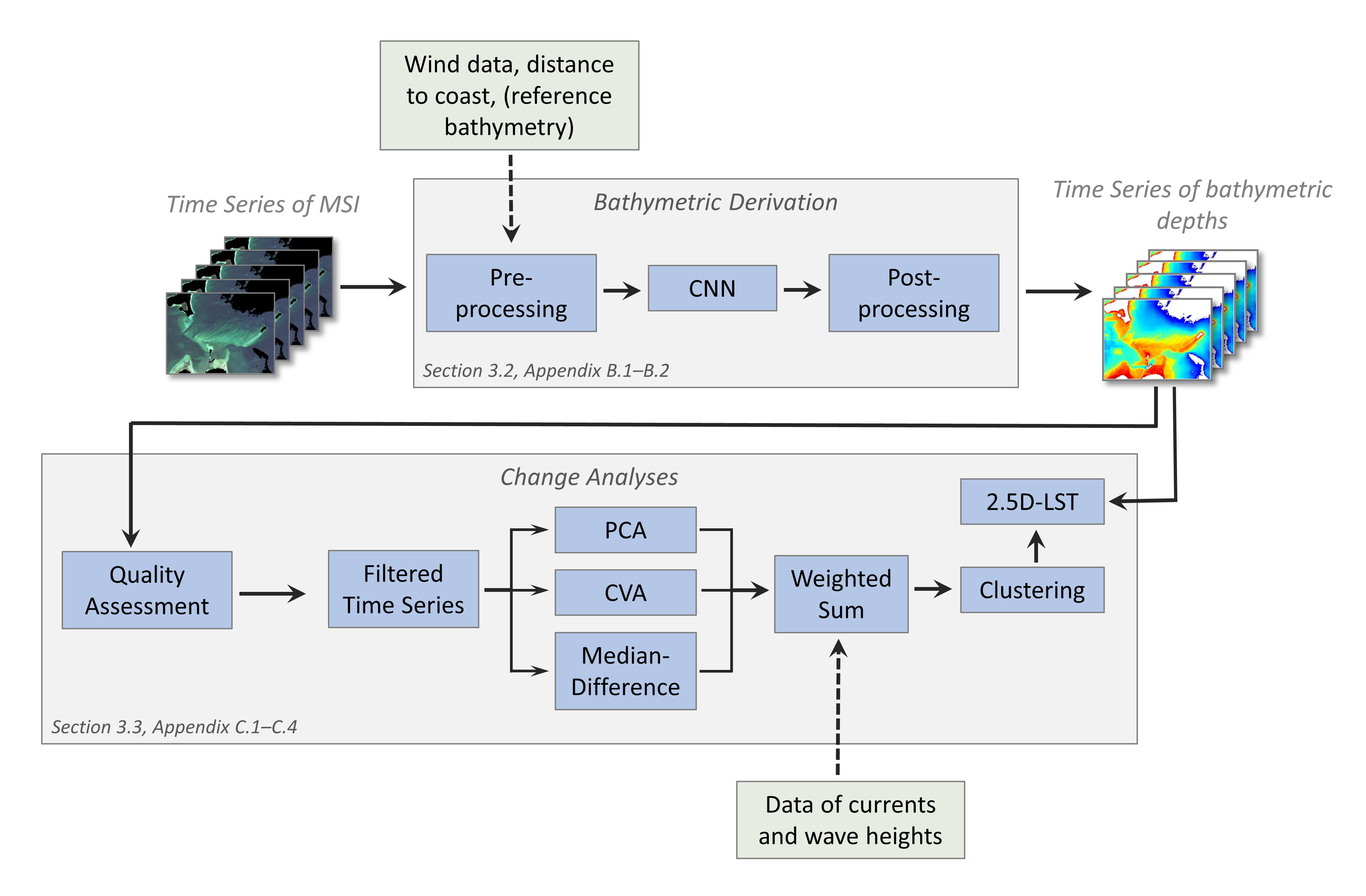
The presented service (Fig. 1) employs a time series of MSI data and supplementary input information (Section 3.1; Appendix A), to initially ascertain the water depths within a specified region. To achieve this, the MSIs are subjected to a pre-processing and pre-sorting operation, after which the bathymetry is computed using a CNN and subsequently undergoes a post-processing phase (Section 3.2; Appendix B). The change analysis (Section 3.3; Appendix C) is performed by first selecting the appropriate MSIs using a quality analysis. Subsequently, the changes are quantified through the utilisation of assorted change detection techniques, the outcomes are merged and clustered in accordance with the traffic light-inspired scheme.

3.1 Used data

Satellite imagery. The proposed service is based on Sentinel-2 data (ESA, 2024) due to its high spatial resolution of up to 10 m × 10 m and the availability of the data at no costs. The Sentinel-2 mission is operated by the European Space Agency (ESA) and currently compromises three satellites (launched in 2015, 2017 and 2024) with a revisit time of ten days for each satellite. The images captured by the satellites possess 13 spectral bands B, five of which, spanning from coastal blue (B₁) to very NIR (B₅), are capable of at least partial penetration into the water body. However, the other bands in the spectrum of NIR and short-wave infrared (SWIR) support the deviation of additional features such as algae, clouds and the land-water-mask (Section 3.2). Images with atmospheric correction and bottom-of-atmosphere (BOA) reflections, generated by the Sen2Cor processor as specified by Louis (2021), are employed for the service.

Bathymetric reference. To generate the CNN for the bathymetric deviation, a data-driven machine learning approach requires reference data on water depth. The data are obtained from multibeam and single-beam echosounder measurements from BSH hydrographic surveys. A 10 m × 10 m raster dataset has been generated from the latest available data, but there is still a time lag between the reference data and the satellite images. Therefore, especially in dynamic areas, they may be outdated and thus incorrect ‘reference’ data. Nevertheless, the aforementioned areas are of a relatively limited extent in comparison to the appropriate areas, thus allowing for the continued utilisation of the data for the training of the CNN.

Additional data. The service employs supplementary data, including wind information, to evaluate the appropriateness of satellite imagery and the distance from the coast to facilitate bathymetric derivation. Additionally, wave height and current ancillary data are integrated, as they are important environmental factors driving seabed variability. Further details regarding the utilised datasets can be found in Appendix A.

3.2 Bathymetric processing workflow

This section covers the steps from the provision of satellite imagery to the bathymetric time series that serve as the basis for the subsequent change analysis (Fig. 1).

In order to ensure the accuracy and reliability of bathymetric calculations derived from satellite imagery, it is of paramount importance to select images that are optimally suited to the prevailing environmental conditions. Factors such as clouds, cloud shadows, atmospheric conditions, turbidity, swell, sun glint, turbidity, foam, algae and ice must be considered to guarantee the precision of the resulting bathymetric data. These challenges are offset by a number of compensatory measures. At the level of the 100 km × 100 km Sentinel-2 images, the sorting process employs cloud masks and wind strength (correlated with turbidity, waves and foam ridges). Moreover, the satellite images are divided into sub-scenes of approximately 20 km × 20 km, with the cloud coverage calculated for each of these sub-scenes. The sub-scenes are then processed to remove any areas designated as land, ice, and foreign territory, after which they are evaluated for suitability (Appendix B.1). In the event that a sub-scene is to be calculated, then turbidity parameters and logarithmic band combinations, as proposed by Geyman & Maloof (2019), are calculated. Due to the computational limitations of the CNN, the sub-scenes are reduced to a smaller size of 256 px × 256 px. Further details on the pre-processing can be found in Appendix B.1.

The subsequent phase is the actual estimation of the bathymetry, which is conducted through the utilisation of CNN regression. CNNs constitute a subset of artificial neural networks (ANN), which are particularly well suited to image analysis due to the presence of built-in spatial filters (LeCun et al., 1998). The CNN is a wholly empirical approach, whereby the relationship between input variables and output bathymetry is learned from reference data without any physical background knowledge. Nevertheless, some physical principles are integrated through the inclusion of input parameters such as the turbidity parameters and the logarithmic band combinations. This work employs the CNN architecture developed by Żak (2020) and utilises a U-net structure (Appendix B.2). The latest model was trained for 80 epochs using 10,000 pre-processed images, as previously described, with 80 % allocated for training and 20 % for validation. The final result of the training process is a bathymetric model with a particular focus on the German Baltic Sea. During the prediction process, the trained model can be employed to derive the water depth from similarly pre-processed small images of new satellite MSI.

The bathymetric result of the CNN has a shape of 256 px × 256 px, which can be reasonable reassembled into a larger and more convenient size of sub-scenes covering an area of approximately 20 km × 20 km. This approach offers a suitable compromise between a comprehensive coverage and the avoidance of unnecessary expansion of the dataset with irrelevant areas such as land and deep waters. The boundary regions of the predicted scenes frequently exhibit considerable deviations due to the limited padding possibilities of the CNNs. Consequently, the prediction is performed with a substantial overlap (~ 80 % has proven useful). For reassembly, the border regions are trimmed and the inner regions are arithmetically averaged.

3.3 Change analysis workflow

The second step in the development of the service is the robust and reliable detection of seabed changes (Fig. 1). This involves the identification and quantification of changes in spatially delimited areas. The input is based on the previously derived time series of bathymetric data.

A qualitative analysis of the derived time series is initially conducted to evaluate the suitability of each time point. Parameters such as cloud cover, wind speed, mean turbidity and the mean difference of the bathymetry from the mean bathymetry are considered to derive an overall score that allows for the adaptive filtering of the time series. Further information may be found in Appendix C.1.

Secondly, a set of change detection techniques are applied to this filtered time series, with each pixel quantified according to its variability over the image series. Thus, a PCA, a CVA and a robust median difference are performed, with each producing one or more parameters describing change. Additionally, another change-describing value is calculated using the wave and current data in the time period under consideration. Further information may be found in Appendix C.2.

The change values are normalised, weighted and summed up to a total change value per pixel. This is then clustered using a k-means algorithm and transferred into four classes, ranging from 0 (no change) to 3 (very strong change). This is followed by morphological filtering to reduce noise. Further details can be found in Appendix C.3.

2.5D LST, an integrated matching technique developed by Westfeld (2012), estimates pixel-wise 3D motion vectors with subpixel accuracy between surface elements of a consecutive image sequence. It employs depth and intensity values in order to fully exploit the potential of the measurement signal, thereby providing a more accurate and reliable solution, particularly in instances where the contrast ratio within one of the two channels is challenging. 2.5D LST is applied to each pixel (and its surrounding 31 px × 31 px neighbourhood, corresponding to 620 m × 620 m on the seabed’s surface) of areas previously identified as being subjected to significant change. Further information can be found in Appendix C.4.

4. Case studies

4.1 Study areas

The case studies employ two distinct areas to evaluate SDB and to examine the change analysis. The SDB evaluation is optimally conducted in a static setting while the change analysis necessitates a dynamic environment. The study area for the bathymetric processing workflow (Section 3.2) is located in the eastern German Baltic Sea in the Bay of Greifswald (German: Greifswalder Bodden; Fig. 2). It is characterised by large areas of shallow water with some deeper shipping lanes in between. Most of the seabed is covered with light-coloured sand and gravel, but there are also areas covered with vegetation that appear dark in the satellite images.

The study area for testing the developed seabed change analysis (Section 3.3) is located north of the Fischland-Darß-Zingst peninsula in the German Baltic Sea (Fig. 3), at a location subjected to very dynamic coastal erosion processes known as “Darßer Ort”. The seabed is dominated by light sandy sediments, with some vegetation to the east, which appears as dark areas in the satellite image. There is an emergency harbour in the eastern part of the peninsula and its access routes are regularly dredged.

4.2 Spectrally-derived bathymetry results and accuracy analysis

The reference data needed to evaluate the bathymetric results were obtained from ship-based single and multibeam echosounder surveys conducted in the study area between 2013 and 2020. The echosounder data were used to generate a raster dataset with a resolution of 10 m × 10 m. The accuracy of the reference water depth data is a few centimetres, but within the interpolated area the deviations may be greater.

For the study case, the developed workflow described in Section 3.2 is tested and the results and accuracies achieved are evaluated. As input information, a bathymetric image is generated from the Sentinel-2 satellite image of 23 June 2019. During post-processing, depths less than 0.25 m were not considered for accuracy analysis, as these very shallow areas are not adequately represented in the reference data used for training, and SDB from very shallow areas is highly susceptible to errors caused by wave breaking. Data from areas deeper than 10 m were also not considered for the accuracy analysis, as the visibility conditions in the Baltic Sea generally do not allow analysis at greater depths (Section 2.1). The bathymetric results obtained are shown in Fig. 4. The characteristics of the seabed are well represented by the estimated bathymetry: Shipping lanes, sandbanks and the ripples on the sandbanks are clearly visible. However, particularly in deeper areas such as shipping lanes, there are systematic errors due to underestimation of water depth (Fig. 4). In addition, the use of 256 px × 256 px images for the CNN induces small raster biases of ~30 cm difference that cannot be adequately addressed by post-processing when merging the small images to the ~ 20 km sub-images (Section 3.2). The magnitude of these raster effects increases with increasing depth of penetration into the water body, due to the depth-related increase in uncertainty associated with the estimation of bathymetry (Section 2.1). The histogram of Fig. 5 illustrates the distribution of the deviation between the reference data and the SDB results, demonstrating a slight systematic underestimation of the bathymetric results with a median deviation of 26 cm (Table 1). Additionally, the results were obtained with a median absolute error (MedAE) of 47 cm, a RMSE of 86 cm, and a 95^th percentile of 1.74 m.

The stated parameters describe the degree of accuracy with which the depth of the German Baltic Sea can be determined from Sentinel-2 MSI at any given time. As a consequence of the constraints imposed by the trained CNN model (Section 3.2), it is not possible to extend the quality metrics to other regions and/or other imaging sensors. The accuracy levels attained are inadequate to fulfil the requirements of Order 1b or better of the IHO S-44 hydrographic survey standard (IHO, 2022), and thus cannot be considered a direct replacement for high-accuracy hydrographic surveying. However, they are available in high temporal resolution and thus constitute an appropriate basis for change analysis, as intended for use in the operational service. Moreover, some systematic deviations are minimised due to the inherent differencing during change analyses (Section 3.3).

4.3 Change analysis

4.3.1 Seabed change monitoring results and accuracy analysis

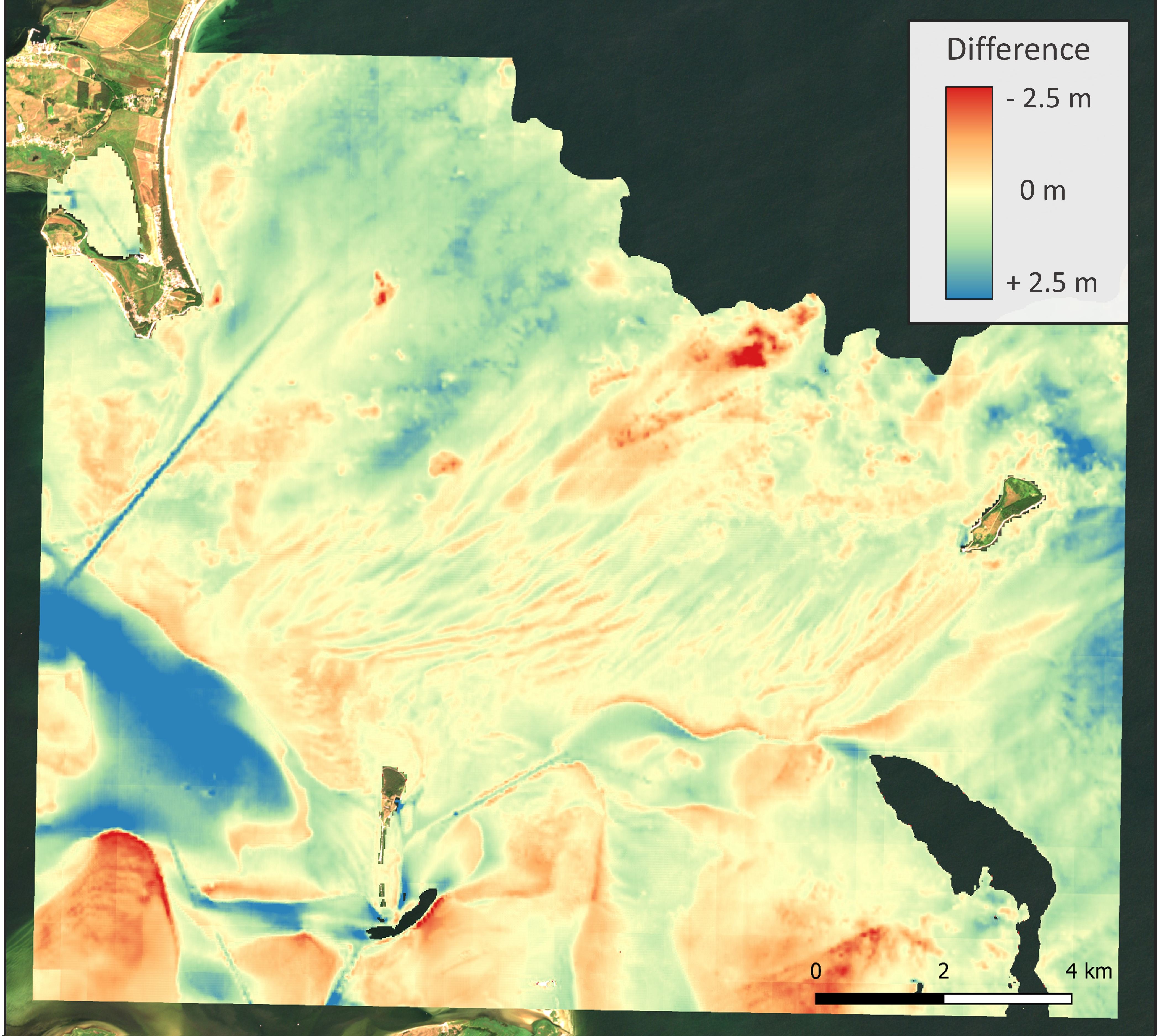
In order to evaluate the results of the change analysis, single-beam echosounder surveys were conducted at Darßer Ort in the spring of 2018 and 2022. The two measurement campaigns were conducted to a minimum depth of 1.5 m. The datasets were processed using the standard workflow employed by the BSH survey division, which consisted of sound speed correction, outlier removal, flagging vegetation, a Delaunay triangulation between the profile tracks and gridding. Two DTMs of the seabed with a resolution of 10 m × 10 m were ultimately produced. The difference between the two DTMs was calculated to determine a reference for seabed variations, as shown in Fig. 6.

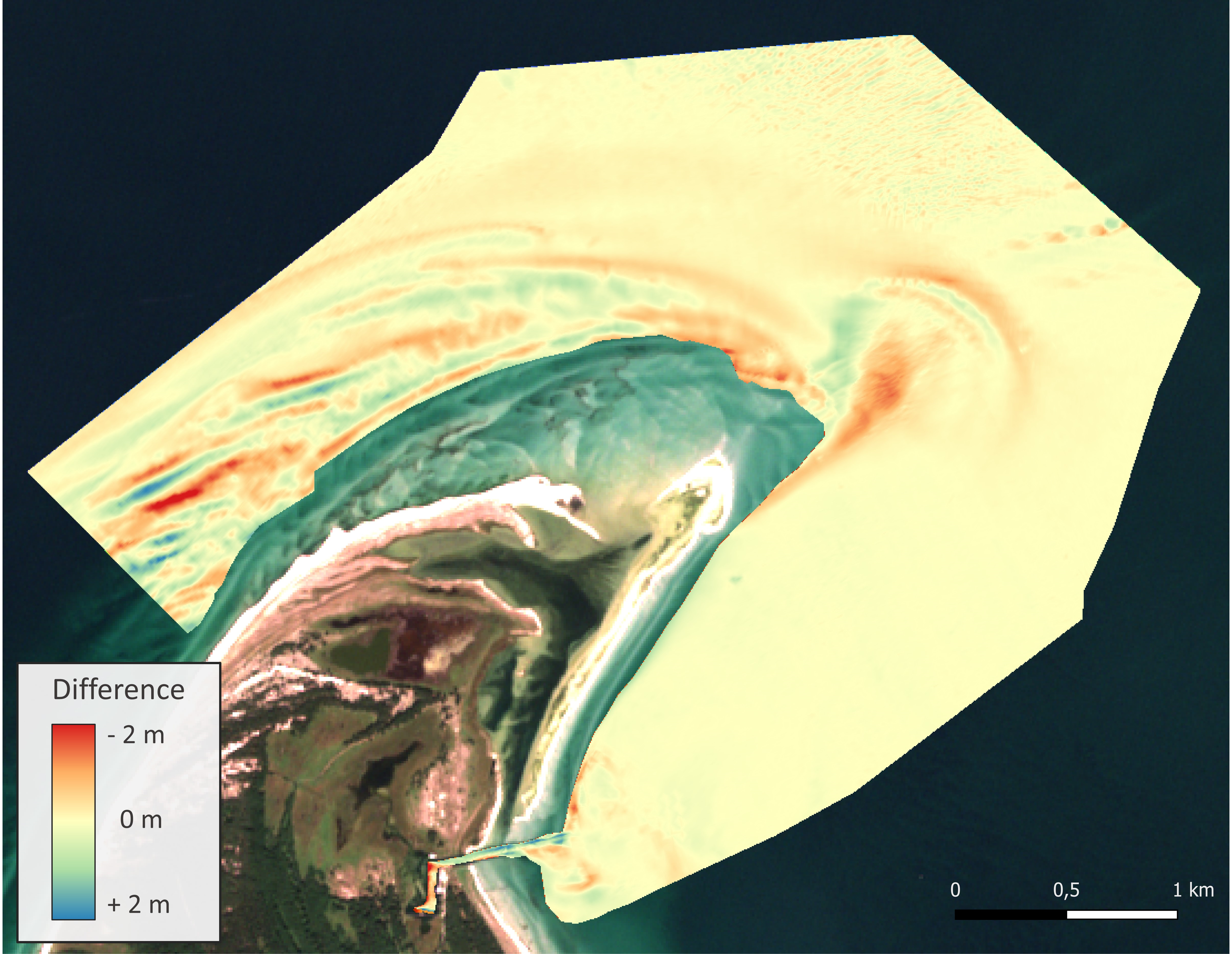
The analysis is based on 43 Sentinel-2 MSI of the study area, acquired between 2018 and 2022. The bathymetry was calculated for these 43 epochs (Section 3.2). In the subsequent quality assessment, 26 epochs were excluded from the analysis (due to the presence of clouds and turbidity, among other factors). The remaining 17 epochs were used as the basis for change analysis. However, the resulting estimate of change is currently expressed as a unitless metric. In order to facilitate comparison with the reference change, both the reference data and the estimated change data have been normalised to a unitless scale between 0 (no change) and 1 (maximum change) using min-max normalisation with the 2.5^th percentile as the minimum and the 97.5^th percentile as the maximum. This approach was employed to reduce the influence of outliers. The results are normalised change intensity values presented in Fig. 7, which demonstrates that the estimated changes exhibit considerable variation in the coastal areas to the north-west and north-east of the peninsula and on the harbour access route in the south-east of the scene. The reference change also displays some corresponding areas of high change, although the areas are subtly different and the change is more clearly delineated, with less background noise.

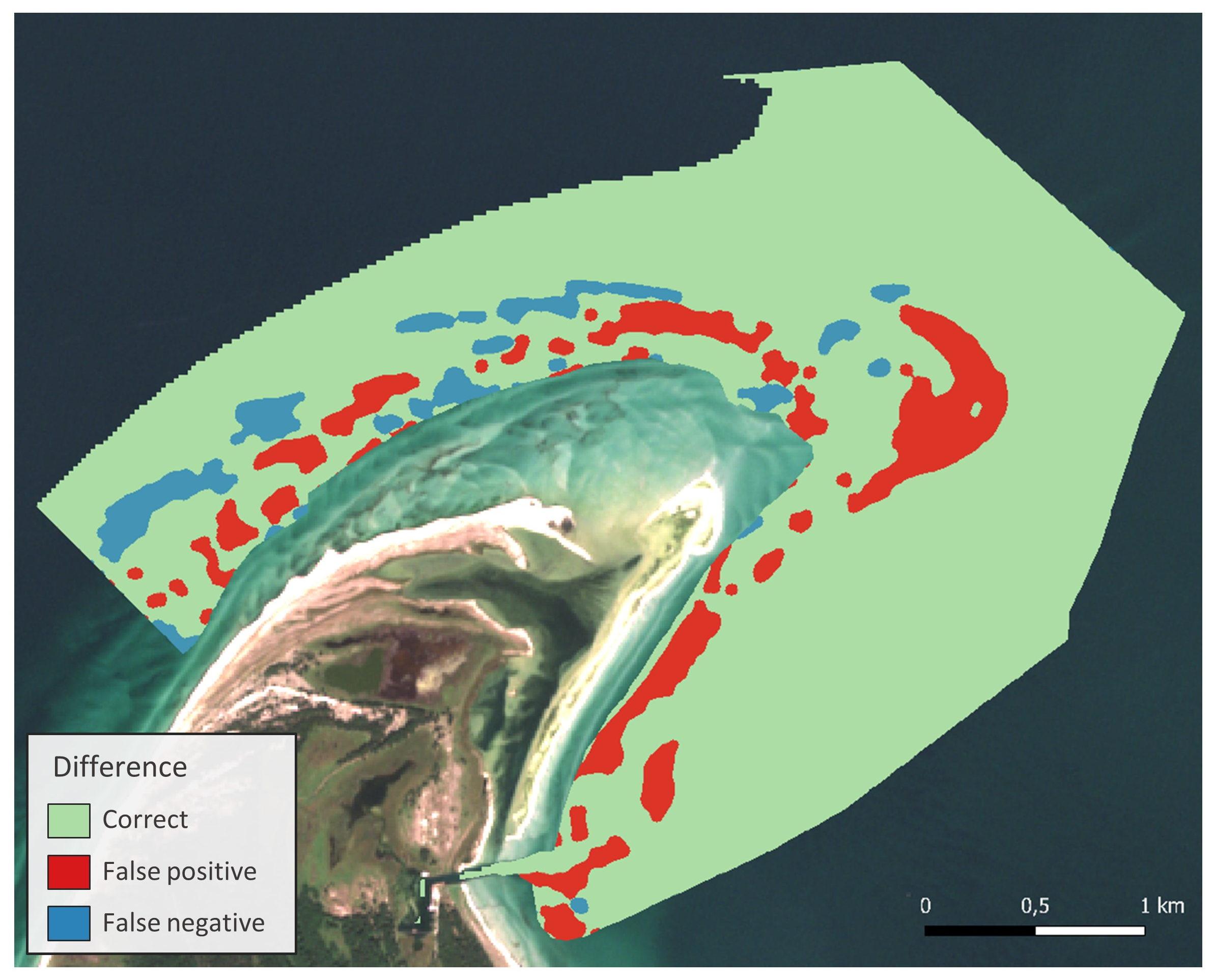
Subsequently, the normalised change values were classified into two categories: change and no change. This differs from the clustering workflow described in Section 3.3, as the clustering algorithm cannot be applied similarly to the reference data. Further, a morphological filter was employed to reduce the influence of small filigree structures and the result is shown in Fig. 8. Afterwards, the discrepancy between the two representations was determined (Fig. 9), allowing the differences between the reference and the calculated seabed variation to be quantified. The majority of 85.0 % of the area shows no deviation between the reference and the estimated data, thereby providing substantiation for the appropriate classification. The occurrence of false positive misclassifications, whereby a change is identified when none exists, is 10.5 %. Conversely, false negative errors, where no change is detected despite the presence of one in the reference data, occur at a frequency of 4.5 %. The accumulation of false positive classifications is evident in areas of the south-east peninsula. Such occurrences are attributed to pronounced variations in reflectance, which are presumed to be the result of transient vegetative accumulations, with a high probability of being seaweed. The aforementioned vegetation deposits have resulted in erroneous entries in the SDB, leading to the misrecognition of changes. Furthermore, instances of distributed misclassifications are more prevalent in the north-western region of the peninsula. This is due to the fact that the entire area is characterised by considerable variability, which gives rise to the detection of such changes, although the spatial extent of specific changes differs in some areas. This discrepancy may be attributed to the fact that the satellite imagery encompasses the entire time span, thereby rendering the continuous changes less discernible than they would be if only two epochs were considered, as for the reference data. Another potential cause is the challenging and highly variable environmental conditions, which range from extremely turbid and foamy waters to those that are remarkably clear and undisturbed. These conditions render the SDB estimate variable, thus increasing the likelihood of error in the change analysis.

4.3.2 Seabed tracking results and evaluation

Fig. 10 shows the motion vector field estimated by 2.5D LST (Section 3.3) for areas that have been previously identified as undergoing change. The length of the derived motion vectors exhibited a range of 1.5 m to 466 m. The mean standard deviation for all lateral vector components estimated (thus ranging from a few metres up to half a kilometre) can be stated with sub-pixel accuracy, with a value of 0.29 px, which corresponds to 5.9 m on the seabed surface. The mean standard deviation for the estimation of the depth component of the motion vectors is 0.15 m. Median averaged over the entire motion vector range, the 3D motion vectors were estimated with a precision of approximately ⅒ of its lengths.

The reported accuracy values are encouraging when considered in the context of a ground sampling distance (GSD), defined as the distance between pixel centres measured on the seabed’s surface, of 20 m (Section 3.2), and an accuracy of 0.86 m for depth value extraction from optical imagery (Section 4.2). It should be noted, however, that these are relative accuracy metrics, as an absolute accuracy analysis cannot be performed due to the lack of reference motion data.

Furthermore, a plausibility check was conducted using time-lapse image sequences of the satellite MSI. The majority of the derived motion patterns were adjudged to be reasonable. The area west of the peninsula is characterised by a uniform motion vector field oriented towards the south-west (Fig. 10, left). This phenomenon can be attributed to the influence of strong currents in easterly winds, which exert a less pronounced effect on the area in the presence of westerly winds. The magnified extract (Fig. 10, right) depicts the peninsula’s tip and shows a motion vector field that is subjected to rotational effects caused by interactions between strong easterly currents and prevailing westerly winds. However, there are also areas with seemingly turbulent motion vectors, dominant especially in the south-east of the peninsula. This phenomenon can be attributed to the distinctive characteristics of the seabed in this region, which is characterised by the presence of marine vegetation. Consequently, in addition to tracking seabed motions, the monitoring also encompassed the tracking of organic material.

5 Towards a fully automated operational service

The objective is to implement a fully automated service that will necessitate the implementation of extensive automation and control of the individual processes. It is imperative that the system is able to accommodate a diverse range of scenarios, encompassing the routine execution of the SDB and change analysis workflow (Sections 3.2 and 3.3) for the entirety of the area under the purview of BSH, as well as manually initiated sub-processes for specific areas and timeframes.

Accordingly, a modular and extensible approach was adopted, with each component of the workflow encapsulated in a separate module class that implements a self-designed interface for configuration and execution. The interface stipulates that each module must provide a dictionary of named parameters that can be employed for configuration purposes, accompanied by the relevant default values. Subsequently, these values may be modified as required and transmitted to the module prior to the initiation of processing. Moreover, this allows the scheduling component to override parameters in a predefined workflow for the execution of a specific task.

The aforementioned modules can be employed either as standalone entities or in conjunction with other modules for the development of workflows. This involves chaining of module executions, whereby the output of one module is used as input for the next. This facilitates the straightforward replacement of specific workflow components with alternative algorithms and data sources in the future.

It is imperative to ensure that the MSI input data is preserved in standardised and predefined formats. Consequently, all satellite images, irrespective of their original format, are transformed into an open, platform-independent GeoPackage format (GeoPackage, 2024) with predefined names for the band layers and the file itself, as well as predefined metadata. This ensures the compatibility of the developed service with imagery from other satellite missions, necessitating only minor modifications to the algorithms implemented. The supplementary data, which includes reference depths, distances to the shore, currents and wave heights, is provided in the form of a Network Common Data Form (NetCDF4, 2024). This is also employed for the resulting output data. Additional data, such as wind data or current data, are downloaded, pre-processed and stored as predefined comma-separated values (CSV) by an external process on a daily basis.

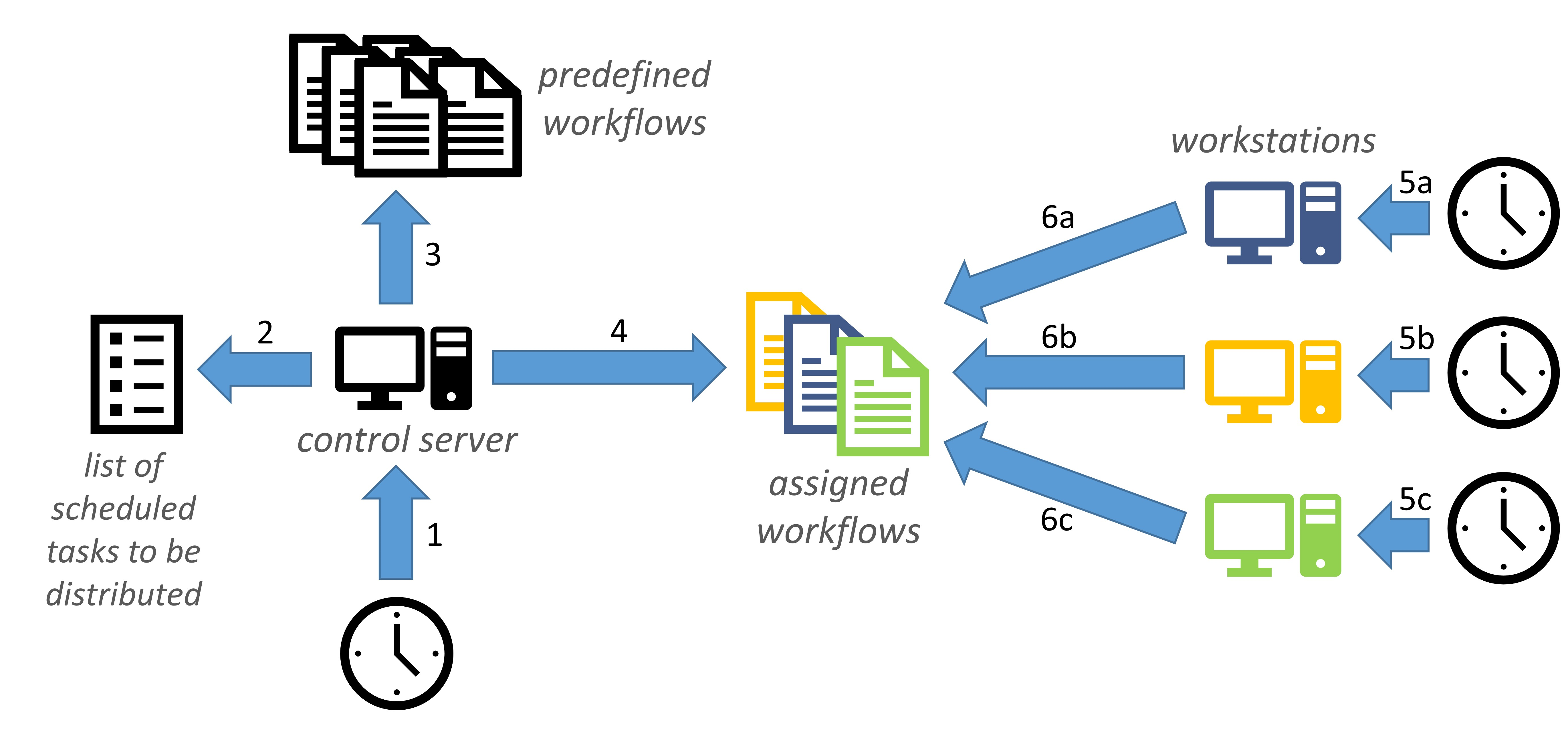
The scheduling process and an overview of the task assignment functionality are illustrated in Fig. 11. Based on a timer (1), the control server is executed on a daily basis and works through the list of scheduled tasks (2), for example, the daily execution of the entire SDB and change analysis. Consequently, the control server retrieves the pertinent workflows (3) and deposits the scripts of a workflow at a known location (4). The designated computers have access to the same data pool on a network drive and are programmed to perform a daily check (5a–5c) for any new tasks assigned to them, by searching for assigned workflows (6a–6c). The workstations responsible for executing the required tasks are standard staff computers, which typically perform these operations at night to minimise interference. The entire workflow is written in Python; however, the activation scripts are shell or batch scripts that are called via cron jobs (Linux) or the Task Scheduler (Windows).

6 Discussion

In light of the significant financial implications associated with the deployment of advanced hydrographic surveying techniques, such as shipborne hydroacoustic or airborne LiDAR technology, the imperative for event-driven resurveying remains. The present study demonstrates that the detection of varying regions of the seabed is feasible through the analysis of MSI sequences using SDB. The developed service is currently operational as a prototype in the German Baltic Sea, monitoring changes in the seabed down to a water depth of 10 metres, which represents approximately 25 % of the BSH’s area of responsibility in the Baltic Sea. This has the potential to result in significant savings in the future, as shallow water areas are typically both highly dynamic and costly to survey due to the necessity for smaller multibeam echosounder line spacings.

The calculation of SDB water depth is of paramount importance. The accuracy of the bathymetric results is influenced by a number of environmental factors, including cloud cover, turbidity and algae, foam crests, seabed habitat and the sun elevation angle. These are discussed in Section 2.1, while Section 3.2 outlines the countermeasures taken by the service to address these issues. However, the impact of these disturbances on reflectance is not fully compensable, resulting in erroneous outcomes. Nonetheless, the accuracy of the SDB in the case study presented in Section 4.2 was achieved with a median absolute error (MedAE) of 0.47 m and a root mean square error (RMSE) of 0.86 m, which is comparable with state-of-the-art SDB methods (Section 2.1). Furthermore, the change analysis eliminates permanent systematic errors in the SDB by considering the differences over time. Consequently, a limited systematic underestimation of large water depths (e.g. in the shipping lanes in Fig. 4) is less problematic, assuming that this underestimation is consistent over time. However, errors that occur only in individual images and vary over time, usually due to the environmental influences mentioned above, present a challenge for the subsequent change analysis.

The findings of the study, as detailed in Section 4.3.1, indicate that the service, which is still in the prototype phase, is capable of accurately classifying a significant portion of the area (approximately 85 %) in accordance with the specified change. This represents a promising initial outcome. However, the service exhibits a tendency to erroneously classify a considerable proportion of areas as bathymetric seabed changes. This is evidenced by the aforementioned study, which identified approximately 10 % of false positives and 5 % of false negatives, and is further corroborated by empirical testing conducted during the development phase. This is primarily due to significant alterations in reflectance that are not accompanied by corresponding changes in water depth, which the SDB workflow is currently unable to capture. Consequently, these “undesirable” changes are identified by the change detection algorithms and can only be partially distinguished from the desired variations in seabed topography. The most challenging aspect is a long-term change in reflectance (without bathymetric change), which is typically caused by changes in the seabed habitat. These changes may include the growth or dieback of seagrass fields, deposition or washing of seaweed, and other factors. In order to compensate for this, it is necessary to identify the location of (or, ideally, to correct) the affected area prior to undertaking a change analysis, as it is not possible to make a compensation during the change analysis itself. Furthermore, recurring or periodic radiometric differences resulting from seasonal vegetation cycles, such as seagrass, kelp forests or algal blooms in bays with minimal water exchange, represent a significant challenge. In order to achieve full compensation of the periodic variations, a dense time series covering the total period, which is usually annual, is required. However, this is not currently feasible, as the most suitable images are generally available only in the summer months, and there are significant data gaps during winter. Additionally, the periods in question are not strictly annual, as growth patterns are influenced by weather conditions, resulting in fluctuations. An alternative approach to addressing this issue is to limit the use of images to those captured during the same time of year. However, this significantly reduces the number of available image sequences. Furthermore, areas that are subject to significant and persistent fluctuations in reflectance present a challenge. This encompasses the coastal surf zone, where turbidity, foam ridges, vegetation deposits, and potential bathymetric changes can all contribute to challenges in data interpretation. The restricted availability of undisturbed satellite images in these regions gives rise to a considerable degree of variability over a given period. Consequently, the change analysis frequently identifies these regions as exhibiting significant variations. This limitation can be addressed by selecting images on days with minimal wind activity. However, the majority of the observed spectral variability in most areas is characterised by one-off (or infrequent) short-term changes caused by factors such as turbidity, atmospheric conditions, waves, sun glint and ship traffic. These effects are largely accounted for by the use of time series information in the change analyses, which incorporates the inherent averaging and median formation, as well as the deliberate image selection during the quality assessment (Section 3.3). These measures also serve to mitigate, at least in part, the effects induced by the periodic and very frequent changes described above.

In order for a change to be reliably identified by the presented service, it must satisfy a number of prerequisites. In the first instance, the change in question must exceed a specific size threshold. The currently employed resolution of 20 m and the settings for morphological filtering during clustering (with the currently used kernel size of 3 px × 3 px) are the determining factors, resulting in a required minimum affected area size of 60 m × 60 m. Furthermore, the change must be discernible for a certain period of time. Nevertheless, it is not feasible to make a universal assertion in this regard, as the accessibility and quality of the satellite images exert a considerable influence. The current parameter configuration necessitates the capture of the change in two to five satellite images, contingent on the magnitude of the change. While this figure could be reduced, this would result in a greater number of areas being incorrectly identified as having undergone change. This is because it is not possible to exclude short-term false values (due to atmospheric conditions, ships, turbidity, etc.). Ultimately, a certain degree of seabed change is necessary, contingent on the precision of the SDB in the region. It is not possible to make a blanket assertion, given that systematic errors in the SDB are partially offset by differencing. However, a change of at least a few dm was typically required during developmental testing.

The fully automatic detection of bathymetric changes, which requires the workflow to be extremely robust, remains a challenge. However, it has been demonstrated that the service is capable of detecting variable areas (Section 4.3) and therefore represents a valuable additional asset in hydrographic survey planning. This is due to the fact that the service is provided free of charge and is fully automated, resulting in negligible financial and personal costs.

7 Summary and outlook

The objective of this research was to develop a prototype service capable of identifying changes in seabed topography based on the spectral data obtained from the Sentinel-2 MSI satellite. The implemented service is fully automated and comprises two distinct phases. The initial phase comprises the estimation of bathymetry through the utilisation of SDB, encompassing the selection of MSI in consideration of cloud cover and wind conditions, a preliminary processing stage (including normalisation, cropping, the calculation of turbidity and pseudo depth parameters, supplementary image selection), the derivation of actual depth through a CNN in a U-Net structure, and a post-processing phase. The CNN model was trained using Sentinel-2 images from the German Baltic Sea region and data from the BSH’s echo sounder-based hydrographic surveying. In a case study, a MedAE of 0.47 m and RMSE of 0.86 m were achieved, thereby demonstrating the accuracy of the SDB. The second phase is the change analysis, which can be conducted once the water depth has been estimated at multiple time points. Firstly, a quality assessment of the available images is conducted, enabling the targeted selection of images. Subsequently, a series of change detection techniques (PCA, CVA and robust difference) are applied to the image sequence with the objective of determining parameters that characterise the dynamics of an area. These parameters are then combined into a weighted sum, clustered and converted into an intuitive traffic light scheme with a recommendation for action. In a field study, 85 % correct classification between areas exhibiting change and those exhibiting no change was achieved. The service provides an estimate of the variability of shallow water areas in advance of a survey. This enables an event-based planning of the resource-intensive hydrographic survey, thereby avoiding the unnecessary repetition of surveys of static areas. Consequently, the allocation of survey resources can be re-prioritised at this juncture, with greater focus placed on dynamic areas to enhance the timeliness of hydrographic survey data. The service, therefore, represents an added value, particularly for hydrographic offices, which can be operated fully automatically and at minimal cost. Furthermore, the service provides comprehensive time series of bathymetric data and change information, which can be employed in environmental monitoring and analogous applications.

At the time of writing, the service is still in a prototype state, and the paper describes the current state of development. In general, the entire workflow is fully operational and produces the results presented. The bathymetry workflow is complete, with the exception of the training of alternative CNN models with modified parameter settings. The change analysis workflow is still undergoing development, revision and optimisation. The fundamental structure of the system remains unchanged; however, the incorporation of additional weights, parameter settings, and algorithms (for change detection or clustering) is still underway. The proposed improvements entail the incorporation of a situational weighting component into the existing static weighting methodology during weighted summation. This component would be calculated on-the-fly with respect to the noise of a summand, measured by the standard deviation of the neighbouring patch or similar parameters. Furthermore, the intention is to integrate the results of the 2.5D LST into the weighted sum, namely the normalised change indicator values. For this purpose, the vector results are to be averaged by magnitude with respect to their direction and converted into rasterised, normalised change information. Furthermore, the integration of current and wave data is intended to be employed for periods exceeding two years through a comparative analysis of the accumulated change activity. This does not permit a general assertion regarding the change; rather, it allows for a comparative assertion within the area under consideration. Furthermore, the integration of additional multi-spectral satellite missions with enhanced spatial resolution is anticipated. Furthermore, enhancing the SDB through the utilisation of local point-shaped data of greater precision, such as crowdsourced bathymetric data or space-borne LiDAR data (e.g. ICESat-2), can prove especially advantageous. The aforementioned data sources are not optimally suited for an area-wide survey, as only a limited number of tracks are measured within a given survey area. However, the data can be employed to ascertain systematic deviations in the SDB, thereby validating the SDB results or even correcting them by an offset, thus performing a local adjustment. This approach would likely enhance the results and increase confidence in the SDB results, thereby indirectly improving the change analysis results.

The accessibility of cost-free remote sensing data has propelled the advancement of satellite-based monitoring programmes and has been progressively acknowledged in the hydrographic community. The advantages of satellite-based monitoring programmes are global coverage, short revisit time and cost-effective data acquisition and analysis. New methods, such as CNNs, optimise the achievable depth accuracies, as demonstrated in this paper. Nevertheless, CNNs are still in the process of being developed, and new modifications, such as physically informed CNNs or multimodal CNNs, which allow the combination of satellite imagery with other data sources, will provide further improvements in achievable depth accuracies. Furthermore, the trend is towards higher resolution satellite imagery and greater computing power, which will further enhance the capabilities of SDB and an SDB-based monitoring programme, as presented in this paper.

Acknowledgements

We gratefully acknowledge financial support of the project Satellitengestützte operationelle Einsatzplanung in der Seevermessung durch integrierte Verarbeitung multispektraler Sentinel-2-Satellitenbildsequenzen (S·O·S) by German Aerospace Center (DLR) with funds from the German Federal Ministry for Digital and Transport (BMDV) under grant no. 50EW2204.

References

Abe, T. (1955). A Study on the Foaming of Sea Water A Tentative Analysis of Wind Wave Data in View of the Foaming of Sea Water. Papers in Meteorology and Geophysics, 6(2), pp. 164–171.

Afaq, Y. and Manocha, A. (2021). Analysis on change detection techniques for remote sensing applications: A review. Ecological Informatics, 63, 101310.

Ahmed, M., Seraj, R. and Islam, S. M. S. (2020). The k-means algorithm: A comprehensive survey and performance evaluation. Electronics, 9(8), 1295.

Asokan, A. and Anitha, J. J. E. S. I. (2019). Change detection techniques for remote sensing applications: A survey. Earth Science Informatics, 12, pp. 143–160.

BSWH (2024). Baltic Sea Wave Hindcast. E.U. Copernicus Marine Service Information (CMEMS). https://doi.org/10.48670/moi-00014

BSWAF (2024). Baltic Sea Wave Analysis and Forecast. E.U. Copernicus Marine Service Information (CMEMS). https://doi.org/10.48670/moi-00011

Braaten, J., Cohen, W. B. and Yang, Z. (2015). Automated cloud and cloud shadow identification in Landsat MSS imagery for temperate ecosystems. Remote Sensing of Environment, 169, pp. 128–138.

Brüning, T., Li, X., Schwichtenberg, F. and Lorkowski, I. (2021). An operational, assimilative model system for hydrodynamic and biogeochemical applications for German coastal waters. Hydrographische Nachrichten – Journal of Applied Hydrography, 118, pp. 6–15. https://doi.org/10.23784/HN118-01

Çelik, O. İ., Büyüksalih, G. and Gazioğlu, C. (2023). Improving the Accuracy of Satellite-Derived Bathymetry Using Multi-Layer Perceptron and Random Forest Regression Methods: A Case Study of Tavşan Island. Journal of Marine Science and Engineering, 11(11), 2090.

Chénier, R., Faucher, M. A. and Ahola, R. (2018). Satellite-derived bathymetry for improving Canadian Hydrographic Service charts. ISPRS International Journal of Geo-Information, 7(8), 306.

Chu, S., Cheng, L., Cheng, J., Zhang, X. and Liu, J. (2023). Comparison of Six Empirical Methods for Multispectral Satellite-derived Bathymetry. Marine Geodesy, 46(2), pp. 149–174.

CODE-DE (2024). Copernicus data and cloud processing for German authorities: CODE-DE. German Aerospace Center (DLR). https://code-de.org (accessed 15 August 2024).

Copernicus Marine Service (2024). Access data. E.U. Copernicus Marine Service Information (CMEMS). https://marine.copernicus.eu/access-data (accessed 9 August 2024).

Deng, J. S., Wang, K., Deng, Y. H. and Qi, G. J. (2008). PCA‐based land‐use change detection and analysis using multitemporal and multisensor satellite data. International Journal of Remote Sensing, 29(16), pp. 4823–4838.

Leder, T. D., Leder, N. and Peroš, J., 2019, Satellite Derived Bathymetry survey method – Example of Hramina Bay. Transactions on Maritime Science, 8(1), pp. 99–108. https://doi.org/10.7225/toms.v08.n01.010

Leder, T. D., Baučić, M., Leder, N. and Gilić, F. (2023). Optical satellite-derived bathymetry: An overview and wos and scopus bibliometric analysis. Remote Sensing, 15(5), 1294.

DWD (2024). Dataset Description. Deutscher Wetterdienst. https://opendata.dwd.de/climate_environment/CDC/observations_germany/climate/hourly/wind/
DESCRIPTION_obsgermany_climate_hourly_wind_en.pdf (accessed 2 September 2024).

ESA (2024). Overview of Sentinel-2 Mission. SentiWiki. https://sentiwiki.copernicus.eu/web/s2-mission (accessed 4 September 2024).

Gower, J., King, S., Borstad, G. and Brown, L. (2005). Detection of intense plankton blooms using the 709 nm band of the MERIS imaging spectrometer. International Journal of Remote Sensing, 26(9), pp. 2005–2012.

Geofabrik GmbH (2024). Download OpenStreetMap data for this region: Germany. Geofabrik. https://download.geofabrik.de/europe/germany.html (accessed 14 August 2024).

GeoPackage (2024). An Open Format for Geospatial Information. Open Geospatial Consortium. http://www.geopackage.org/ (accessed 20 August 2024).

Geyman, E. C. and Maloof, A. C. (2019). A simple method for extracting water depth from multispectral satellite imagery in regions of variable bottom type. Earth and Space Science, 6(3), pp. 527–537.

Haklay, M. and Weber, P. (2008). Openstreetmap: User-generated street maps. IEEE Pervasive computing, 7(4), pp. 12–18.

Hartmann, K., Reithmeier, M., Knauer, K., Wenzel, J., Kleih, C. and Heege, T. (2022). Satellite-derived bathymetry online. The International Hydrographic Review, 28, pp. 53–75. https://doi.org/10.58440/ihr-28-a14

IHO (2022). Standards for Hydrographic Surveys (ed. 6.1). IHO Special Publication S-44, International Hydrographic Organization, Monaco. https://iho.int/uploads/user/pubs/standards/s-44/S-44_Edition_6.1.0.pdf (accessed 29 July 2024).

IHO (2024). Guidance to Satellite-derived Bathymetry (1st ed.). IHO Publication B-13, International Hydrographic Organization, Monaco. https://iho.int/uploads/user/pubs/bathy/B_13_Ed100_032024.pdf (accessed 29 July 2024).

Jégat, V., Pe’eri, S., Freire, R., Klemm, A. and Nyberg, J. (2016). Satellite-derived bathymetry: Performance and production. In Proceedings of the Canadian Hydrographic Conference, Halifax, NS, Canada, pp. 16–19.

Lacaux, J. P., Tourre, Y. M., Vignolles, C., Ndione, J. A. and Lafaye, M. (2007). Classification of ponds from high-spatial resolution remote sensing: Application to Rift Valley Fever epidemics in Senegal. Remote sensing of environment, 106(1), pp. 66–74.

Laporte, J., Dolou, H., Avis, J. and Arino, O. (2023). Thirty years of Satellite Derived Bathymetry: The charting tool that Hydrographers can no longer ignore. The International Hydrographic Review, 29(1), pp. 170–184. https://doi.org/10.58440/ihr-29-a20

Legleiter, C. J., Roberts, D. A. and Lawrence, R. L. (2009). Spectrally based remote sensing of river bathymetry. Earth Surface Processes and Landforms, 34(8), pp. 1039–1059.

Louis, J., Devignot, O. and Pessiot, L. (2021). S-2 MPC – Level-2A Algorithm Theoretical Basis Document. Tech. Rep. S2-PDGS-MPC-ATBD-L2A – 2.10, European Space Agency (ESA), Keplerlaan 1, 2201 AZ Noordwijk, The Netherlands, 2021. https://step.esa.int/thirdparties/sen2cor/2.10.0/docs/S2-PDGS-MPC-L2A-ATBD-V2.10.0.pdf (accessed 22 October 2024).

Lyzenga, D. R. (1978). Passive remote sensing techniques for mapping water depth and bottom features. Applied Optics, 17(3), pp. 379–383.

Mandlburger, G. (2022). A review of active and passive optical methods in hydrography. The International Hydrographic Review, 28, pp. 8–52. https://doi.org/10.58440/ihr-28-a15

Najar, M. A., Benshila, R., Bennioui, Y. E., Thoumyre, G., Almar, R., Bergsma, E. W. J., Delvit, J.-M. and Wilson, D. G. (2022). Coastal bathymetry estimation from Sentinel-2 satellite imagery: Comparing deep learning and physics-based approaches. Remote Sensing, 14(5), 1196. https://doi.org/10.3390/rs14051196

NetCDF4 (2024). Network Common Data Form (NetCDF). NSF Unidata. https://www.unidata.ucar.edu/software/netcdf/ (accessed 20 August 2024).

Poicyn, F. C., Brown, W. and Sattinger, I. J. (1970). The measurement of water depth by remote sensing techniques. Technical Report 8973-26-F, Willow Run Laboratory, The University of Michigan.

Ronneberger, O., Fischer, P. and Brox, T. (2015). U-net: Convolutional networks for biomedical image segmentation. In Medical image computing and computer-assisted intervention–MICCAI 2015: 18th international conference, Munich, Germany, October 5-9, 2015, proceedings, part III 18, pp. 234–241. Springer International Publishing.

Stumpf, R. P., Holderied, K. and Sinclair, M. (2003). Determination of water depth with high‐resolution satellite imagery over variable bottom types. Limnology and Oceanography, 48(1part2), 547–556.

Susa, T. (2022). Satellite derived bathymetry with Sentinel-2 imagery: Comparing traditional techniques with advanced methods and machine learning ensemble models. Marine Geodesy, 45(5), 435–461.

Westfeld, P. (2012). Geometrische und stochastische Modelle zur Verarbeitung von 3D-Kameradaten am Beispiel menschlicher Bewegungsanalysen. Verlag der Bayerischen Akademie der Wissenschaften in Kommission beim Verlag C. H. Beck, München, 281 p., ISBN 978-3-7696-5099-0.

Westfeld, P., Maas, H. G., Bringmann, O., Gröllich, D. and Schmauder, M. (2013). Automatic techniques for 3D reconstruction of critical workplace body postures from range imaging data. ISPRS journal of photogrammetry and remote sensing, 85, pp. 56–65. https://doi.org/10.1016/j.isprsjprs.2013.08.004

Wold, S., Esbensen, K. and Geladi, P. (1987). Principal component analysis. Chemometrics and intelligent laboratory systems, 2(1-3), pp. 37–52.

Xie, C., Chen, P., Zhang, S. and Huang, H. (2024). Nearshore Bathymetry from ICESat-2 LiDAR and Sentinel-2 Imagery Datasets Using Physics-Informed CNN. Remote Sensing, 16(3), p. 511.

Xu, H., Wang, Y., Guan, H., Shi, T. and Hu, X. (2019). Detecting ecological changes with a remote sensing based ecological index (RSEI) produced time series and change vector analysis. Remote Sensing, 11(20), 2345.

Żak, K. (2020). keras-unet. GitHub. https://github.com/karolzak/keras-unet?tab=readme-ov-file (accessed 9 July 2023).

Appendix A: Additional data

Wind data. The presented service employs wind data from a curated set of DWD weather stations situated within or in the immediate vicinity of the German Baltic Sea. These are employed to evaluate the MSI, given that the suitability of satellite images is impaired by strong winds, which result in the formation of waves, foam, and increased turbidity due to sediment swirls. The weather stations directly measure wind speed and direction, and the data are provided on an hourly to a 6-hours basis (DWD, 2024). In order to be included in the service, the daily average wind speed from the nearest weather station to the centre of the respective satellite image is used (Section 3.2).

Distance to coast data. In order to assist the CNN in determining the approximate location of an image (Section 3.2), a dataset comprising the distance from the shore is provided. The dataset has been derived from OpenStreetMap (Haklay & Weber, 2008) shoreline data provided by Geofabrik GmbH (2024). The dataset for the distance to the coast was calculated at a resolution of 10 m × 10 m using the QGIS tool “Proximity (Raster Distance)”.

Wave height information. The Copernicus Marine Service (2024) data on wave height are employed as an independent information source for change analysis. The data set designated “Baltic Sea Wave Hindcast” (BSWH, 2024) and the data set designated “Baltic Sea Wave Analysis and Forecast” (BSWAF, 2024) are employed to obtain the “Sea Surface Wave Significant Height (SWH)”, which is provided on an hourly basis with a resolution of 2 km × 2 km. In order to facilitate the utilisation of the data set within the developed service, the wave heights are aggregated on a daily basis, employing the 85th percentile. Furthermore, the resolution of the wave data is linearly interpolated in order to align with that of the change analysis. Finally, the ratio of the wave height to the water depth is calculated utilising the reference data outlined in Section 3.1, which provides information regarding the water depth information.

Current data. The current data derived from the BSH current forecast is included to serve as an external information source for change analysis (Brüning et al, 2021). The dataset has a spatial resolution of 0.5 nautical miles × 0.5 nautical miles and maps the current velocity in latitude, longitude and depth direction, resulting in a total of 25 depth layers every 15 minutes. The velocity is processed by means of a Euclidean sum across all three directions, an arithmetic average along the depth layers and a reduction in time to the 85th percentile of the day. The spatial resolution is then linearly interpolated to match that of the change analysis.

Appendix B: Processing workflow of the bathymetric deviation

B.1 Pre-processing

To reduce errors related to atmospheric conditions and clouds, a satellite image is only downloaded and processed if the percentage of clouds used by CODE-DE (2024) is below a threshold of 5 %. The objective of this rather strict limit is to mitigate the issues associated with the emergence of thin and barely perceptible veil clouds, which are especially prevalent in images characterised by elevated cloud cover. These clouds give rise to systematic errors in the bathymetric derivation. Furthermore, this reduces errors caused by cloud shadows. Images captured on days with high wind speeds are also sorted according to the weather station in the area. This is due to the fact that periods of high wind speed cause significant seabed visibility problems, namely swell, wave whitecaps and increased turbidity due to sediment turbulence. These factors are therefore excluded from the analysis. The threshold for this exclusion is set at four Beaufort, as this is the wind speed at which widespread foaming begins (Abe, 1955).

When the MSI data is downloaded, it is merged with the reference depth and shoreline distance supplements. It is then downsampled to a spatial resolution of 20 m × 20 m, which empirical studies have shown to be a good compromise between noise reduction and spatial resolution. After this, the original 100 km × 100 km Sentinel-2 images are sliced into smaller sub-images of ~ 20 km with an overlap of ~ 0.5 km. This helps to speed up the calculation process by excluding some sub-scenes because they are mainly on land, in optically deep-water areas or not in waters under the responsibility of BSH. Therefore, a mask is created that marks these non-relevant pixels and excludes them from the evaluation by setting the values to blank value (NaN). During prediction, the ratio of the relevant shallow water pixels to non-relevant pixels should be at least 0.25 %, rejecting only scenes made up of mostly irrelevant pixels. In contrast, the threshold is set at 5 % during the training phase to avoid bloating the number of training images with images showing mostly outmasked areas. Another exclusion of these ~ 20 km sub-scenes is caused by the cloud cover. Here, we use the cloud detector of Braaten et al. (2015) and an exclusion threshold of 10 %, which was found in empirical studies and is active during the training and prediction phase.

For the remaining sub-scenes in the un-masked area, we calculate various parameters describing water turbidity and algae such as the Normalised Difference Turbidity Index (NDTI; Lacaux et al., 2007), the Maximum Chlorophyll Index (MCI; Gower et al., 2005), the Green Normalised Difference Vegetation Index (GNDVI; Buschmannm & Nagel, 1993) and the hue angle. These parameters help to mitigate the influence of water quality through the CNN. Furthermore, we derive several logarithmic band combinations, inspired by Geyman & Maloof (2019), such as the band combinations between blue-green, blue-red, blue-NIR, green-red, green-NIR and red-NIR to support the link between spectral information and water depth. For the calculations in this paper, the scenes were reduced to a size of 256 px × 256 px containing 16 bands with the reference depth, the spectral bands B1–B5, the logarithmic band combinations, the turbidity parameters and the shoreline distance.

B.2 Bathymetric regression with CNN

The CNN architecture employed was developed by Żak (2020) and adopts a U-net structure, characterised by a contracting path (encoder) and an expanding path (decoder), as introduced by Ronneberger et al. (2015). The U-Net comprises multiple depth layers, formed by progressively downsampling the input image in the encoder path, extracting increasingly abstract features, and then upsampling in the decoder path to produce a full-resolution result. Each depth layer of the encoder compromises of a batch normalisation, followed by a 2D convolution, a 2D max-pooling, another batch normalisation, a 2D convolution, a batch normalisation, and a final 2D convolution with spatial resolution reduction. In contrast, a depth layer of the decoder is constituted by a concatenation operation with the corresponding encoder level, a batch normalisation, a 2D convolution, a batch normalisation, a 2D convolution, a batch normalisation and a transposed 2D convolution, which serves to restore the spatial dimensions. This architectural configuration enables the network to capture both local and global context. Training a CNN for SDB requires a sufficient amount of different training data that represent the expected variability in, among other factors, the atmosphere, turbidity, subsurface conditions, wave action and solar radiation. The estimation of water depth from new satellite imagery can only be reliable for those areas that have been included in the training data. For the results presented in this paper, the CNN was created using five depth layers, the “Rectified Linear Unit (ReLU)” as activation function, the “Adaptive Moment Estimation (Adam)” as optimiser, the “Mean Square Error (MSE)” as loss function and a batch size of 128.

Appendix C: Processing workflow of the change analysis

C.1 Quality assessment

The objective of the quality assessment is to select the images that exhibit the optimal environmental conditions, which are likely to result in the most precise bathymetric data, for change analysis. To this end, a series of quality parameters are compiled and analysed for each approximately 20 km sub-image. The parameters listed below are absolute values, with a calculated relative value that may not always be meaningful. For instance, the mean absolute turbidity value of a sub-image cannot be interpreted, but a temporal comparison in the same area can highlight points of lower turbidity. The following relative values are then used to generate scores to assess the suitability of the sub-images:

Score_Clouds: The averaged relative cloud cover values for the full Sentinel-2 image, as found in the image attributes metadata, and for the sub-image, which was calculated using the cloud mask methodology proposed by Braaten et al. (2015).

Score_Turb: The average of the relative values of the sub-image mean of the “turbidity” values NDTI and GNDVI.

Score_Bathy: The relative value of the mean difference between the bathymetry of the sub-image and the median bathymetry of the sub-image sequence.

ScoreOther: The average of the relative wind and the relative land percentage.

The individual scores are aggregated to derive an overall score, with the following empirically determined weightings being applied:

(2)

Ultimately, the most appropriate images are selected based on the aforementioned score value. Empirical studies have demonstrated that retaining approximately 40–60 % of images with the highest score value represents an appropriate selection of the image sequence for subsequent change analysis.

C.2 Change detection algorithms

Three change detection algorithms are executed in parallel in order to quantify the change in the time series and thus distinguish between static and dynamic areas using the filtered image sequence described in Appendix C.1.

One method is the PCA (Wold et al., 1987), which is a mathematical method used to reduce the dimensionality of large datasets by transforming a large set of variables into a smaller one that still contains most of the information in the original set. For the following PCA analysis, the time series of length t with two information channels (depth and intensity) are combined to an artificial image with 2 × t bands. These 2 × t bands are highly redundant due to the correlation between the depth and greyscale channels and, more importantly, because many areas have not changed and therefore all t images have the same content in these areas (Deng et al., 2008). The number of principle components (PC) is now determined until a certain percentage of the original information is contained. In previous analyses, a value of around 90–95 % has proved to be adequate. The original time series can now be reconstructed from these PCs, with static areas reproduced very well and dynamic areas much worse due to the loss of information of 5–10 %. To highlight the areas of change the median difference between the original and reconstructed time series is calculated.

The CVA is a widely used change detection technique in remote sensing that calculates the difference vector of the observed features (depth and greyscale) between two time points (Afaq, 2021). The difference vector consists of the magnitude and the direction, indicating the change. When analysing the time sequence, the difference vectors between the adjacent time points are calculated, resulting in t-1 vectors. Tests have shown that the median difference of these vectors is a robust indicator of variable areas.

A robust difference calculation is also performed. In addition to the pre-sorting by the quality assessment, a median image with as little noise as possible is calculated for the given start and end points. For this reason, a division into three parts over time has proved to be successful in tests. The images in the first and last third of the evaluation period are used to calculate the respective median image, while the images in the middle third are ignored. The difference between these two robust, almost noise-free images highlights variable areas.

Furthermore, change information is to be generated from the current and wave data by deriving activity indices for both current and wave data (or more precisely, the ratio of wave height to water depth). To do this, the current or wave activity for each day is assigned to a number from 0 to 10, depending on the current speed or the ratio of wave height to water depth respectively. These values are then summed up for the study period to a single value per pixel which indicates the probability of change due to currents or waves. The absolute value provides information on bathymetric changes in the area independent of the MSI data. However, it is only useful for limited time periods as the summed change value becomes very large in long-term observations due to multiple storm events in the meantime. Therefore, in the current workflow, these change values are only used for observation periods of less than 2 years (found in developmental studies).

C.3 Normalisation, weighted sum, post-processing and clustering

Before combining the results of the individual change detection techniques, the individual results must be normalised. Min-max normalisation is used with the 5th percentile as the minimum and the 95th percentile as the maximum to minimise the effect of outliers. Values that end up less than zero or greater than one are set to zero or one respectively. A weighted sum is calculated to combine these normalised change indicator values, where the weights are predefined with empirically determined values. The resulting summed up change value is then post-processed with respect to the estimated uncertainty of the resulting change value. For areas very close to the coast (< 200 m), a downward weighting is applied to compensate for the effects of strong disturbance of the water column, waves and foam. In addition, a downward weighting is applied with increasing water depth due to the generally decreasing accuracy of the SDB with increasing depth. The same change value is therefore much more reliable in shallow water than in deeper water. Finally, a single total change is derived for each pixel, which is used as input for the clustering and seabed tracking (Appendix C4).

Areas with similar change patterns are clustered and converted into a traffic light inspired scheme. A k-means clustering (Ahmed et al., 2020) is performed based on the total change values, followed by morphological filtering to reduce noise. The k-means model was generated by fitting the derived change values of the entire German Baltic Sea into 12 classes according to their change intensity. This model is now being used in the different sub-areas and time periods. For ease of interpretation, these 12 classes have been combined into four classes ranging from 0 (no change) to 3 (very strong change). As the classification is done pixelwise, there are many fine unrealistic structures with salt-and-pepper noise, which is minimised by morphological filtering.

C.4 Seabed tracking with 2.5D LST

A more detailed motion analysis is conducted using 2.5D LST, which is applied to the areas previously identified as changing. This algorithm enables the pixel-wise tracking of small elements of the surface of the seabed through a sequence of images, thereby inferring the magnitude and direction of seabed motions. 2.5D LST is formulated as an iterative least squares adjustment procedure. The algorithm maps small surface segments of consecutive depth and intensity image data sets on top of one another, with the objective of minimising the sum of the squares of the depth and intensity value differences. This is achieved by estimating eight geometric parameters for translation, rotation, scale, inclination and perspective-related deviation and two parameters for radiometric adjustments (Westfeld, 2013). The input images are selected based on the score value derived from the quality analysis, with a greater weight assigned to images captured at longer time intervals to ensure that the selected images represent the greatest possible temporal range. 2.5D LST provides fully 3D displacement vectors with subpixel accuracy, thus offering a comprehensive representation of seabed topography. This allows for a detailed insight into the dimensions and directions of changes in the seabed.

Authors’ biographies

Since 2022, Peter Grabbert has been employed as a scientific assistant at BSH, the Federal Maritime and Hydrographic Agency of Germany. He holds a Master’s degree in Geodesy from the Technische Universität Dresden, specialising in remote sensing and photogrammetry. During the Master’s thesis and the project at the BSH, he developed an SDB-based change analysis to monitor seabed changes, which runs as an automatic service. He also utilises his expertise in AI applications in remote sensing to host the AI regulars’ table at the BSH.

Mirko Bothe pursued studies in the field of applied computer science, with a specialisation in geoinformatics, at the Georg-August-University in Göttingen. Upon completion of his Master’s degree, he was employed at the University of Rostock as a GIS expert and subsequently as a developer of GIS software for agriculture and UAVs at a small company. In 2019, he was employed in a research and development role within the Hydrography and Geodesy division of the German Federal Maritime and Hydrographic Agency (BSH). His work involves the automation and optimisation of workflows for satellite-derived bathymetry.

Dr.-Ing. Patrick Westfeld graduated as a geodesist from TU Dresden (Germany) in 2005. He conducted research in the fields of photogrammetry and laser scanning and completed his PhD in 2012 on geometric-stochastic modelling and motion analysis. Since 2017, Dr Westfeld has been Head of R&D in Hydrography and Geodesy at BSH, the German Federal Maritime and Hydrographic Agency. The activities of his division range from conceptual issues pertaining to hydroacoustic and imaging sensor technologies, sensor integration and modelling, algorithm development up to application-specific implementation and practical transfer into the production environment.