1 Introduction

Hydrographic Offices (HOs) play a vital role in ensuring maritime safety by collecting hydrographic data and producing authoritative nautical information. In Canada, this responsibility is carried out by the Canadian Hydrographic Service (CHS). Like many HOs, the CHS faces ongoing challenges in maintaining up-to-date hydrographic data across all navigable waters. The vast scale of Canada’s waters, combined with dynamic environments and adverse weather conditions such as seasonal ice, limits the timely collection of traditional survey data. These challenges are most pronounced in the Arctic, where remoteness, harsh conditions, and a short survey season further restrict survey operations.

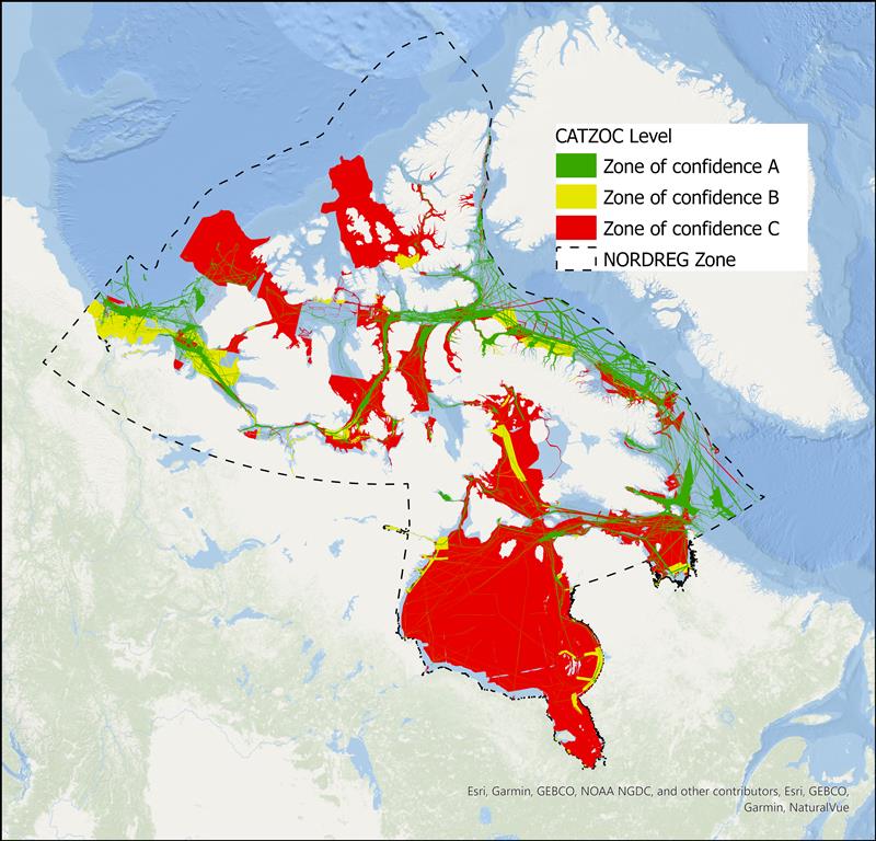
To help address these gaps, the CHS received targeted funding through the Oceans Protection Plan (TC, 2023) to enhance hydrographic data collection in the Arctic. Despite recent advances in modern surveying technologies, only 18 % of the Northern Canada Vessel Traffic Services Zone (NORDREG) is currently covered by surveys meeting modern adequacy standards (i.e., CATZOC A and B), as shown in Figure 1. Areas classified as CATZOC C, while still represented on charts, do not meet current definitions of modern or adequate survey coverage and therefore contribute to the overall gap. This limited coverage highlights the ongoing need for improved data acquisition and the importance of investing in innovative techniques to fill data gaps.

In recent years, the CHS has increased its efforts to integrate remote sensing technologies to supplement traditional survey methods and improve navigational safety. The need to accelerate the integration of remote sensing in the Canadian Arctic has been widely documented (Chénier et al., 2018; Ahola et al., 2020; Chénier et al., 2020a; Chénier et al., 2020b; Chénier et al., 2025; Knudby, 2025). Over the past eight years, the CHS, through the Oceans Protection Plan (OPP), has significantly expanded Arctic data‑collection efforts while investing in remote sensing innovation. Although remote sensing is highly effective for detecting hazards to navigation, the scale of the region – approximately 3.7 million km² – means that considerable work remains to fully identify hazards and update all associated nautical products. To date, regions of high maritime traffic have been screened for hazards using remote sensing and artificial intelligence (Chénier et al., 2018), establishing hazard detection and charting as an ongoing operational activity. The CHS Remote Sensing Centre of Expertise (RSCoE) has made considerable progress in developing methodologies tailored specifically to hydrographic applications (Chénier et al., 2020a), positioning remote sensing as a valuable tool for expanding data coverage. The RSCoE produces a range of satellite‑derived products, including bathymetry, shoreline mapping, intertidal zone delineation, identification of navigational hazards, and change‑detection analyses for monitoring dynamic coastal environments. Among these, Satellite‑Derived Bathymetry (SDB) is particularly significant, as it supports both survey operations and emergency response by highlighting hazardous areas and filling data gaps where traditional survey data are limited or unavailable. Although SDB has been in use for over 50 years (Polcyn et al., 1970), recent advances in multispectral sensors and machine-learning-based depth-estimation techniques have improved its accuracy and reliability.

SDB encompasses several methodological approaches, including photogrammetric methods based on image matching and stereoscopy (Chénier et al., 2016, 2018; Hodúl et al., 2018), and spectral-based techniques derived from multispectral imagery. These spectral-based techniques include both physics-based approaches that model light propagation within the water column (Lee et al., 1999; Mobley, 2022; Lyzenga et al., 2006; Dekker et al., 2011), and empirical methods that estimate water depth from spectral reflectance relationships between bands (Lyzenga, 1978, 1985; Lyzenga & Vid Lyzenga, 1981; Stumpf et al., 2003; Knudby et al., 2016; Kerr & Purkis, 2018). The RSCoE primarily relies on spectral-based empirical approaches due to their simplicity, lower cost, and demonstrated effectiveness in shallow coastal environments.

In this study, SDB refers primarily to the spectral-based empirical approach used operationally within the RSCoE. SDB can be an effective method for HOs to estimate water depths in shallow coastal regions. The CHS began incorporating SDB into its nautical charting workflow in 2018. In June 2018, CHS released its first nautical chart updated using SDB data, Chart 4955 (Havre-aux-Maisons) (Chénier et al., 2018; Chénier et al., 2020a). Since then, CHS has continued to leverage SDB to enhance nautical charting and support mission planning. Empirical methods remain the most frequently used SDB approaches within the CHS RSCoE.

Although SDB offers clear advantages for CHS operations-particularly its ability to address survey gaps with cost- and time-efficient coverage (Chénier et al., 2018; Chénier et al., 2020a; Chénier et al., 2025)—its operational deployment remains constrained by environmental, methodological, and data-related limitations that must be rigorously evaluated to ensure safe and appropriate application in hydrographic contexts.

Within this operational context, SDB is also used to support survey mission planning under strict time constraints. The purpose of SDB mission support is not to create a product suitable for nautical use, but to rapidly generate a preliminary SDB surface that meets the timelines imposed by scheduled field surveys. This preliminary SDB is intended to provide timely depth information to support survey mission planning, guide data acquisition in priority areas, and enhance navigational safety, thereby helping to ensure the safety of survey crews during field operations. To meet these strict timelines, the RSCoE compiles and integrates all available sources of water depth information. Highest priority is assigned to in situ CHS data that have already been calibrated to chart datum, typically Lower Low Water Large Tide (LLWLT). When these data are unavailable or insufficient to fill critical gaps, the RSCoE supplements them with additional sources, including laser altimetry from the Ice, Cloud, and Land Elevation Satellite 2 (ICESat-2) and Crowdsourced Bathymetry (CSB).

Building on this operational context, this paper examines the applications of SDB within a hydrographic framework that prioritizes navigational safety and nautical chart reliability. It presents the iterative approach developed by the CHS RSCoE, emphasizing the practical treatment of accuracy, precision, and uncertainty, and positioning SDB as a complementary input to chart modernization.

2 Methodology

2.1 The iterative process

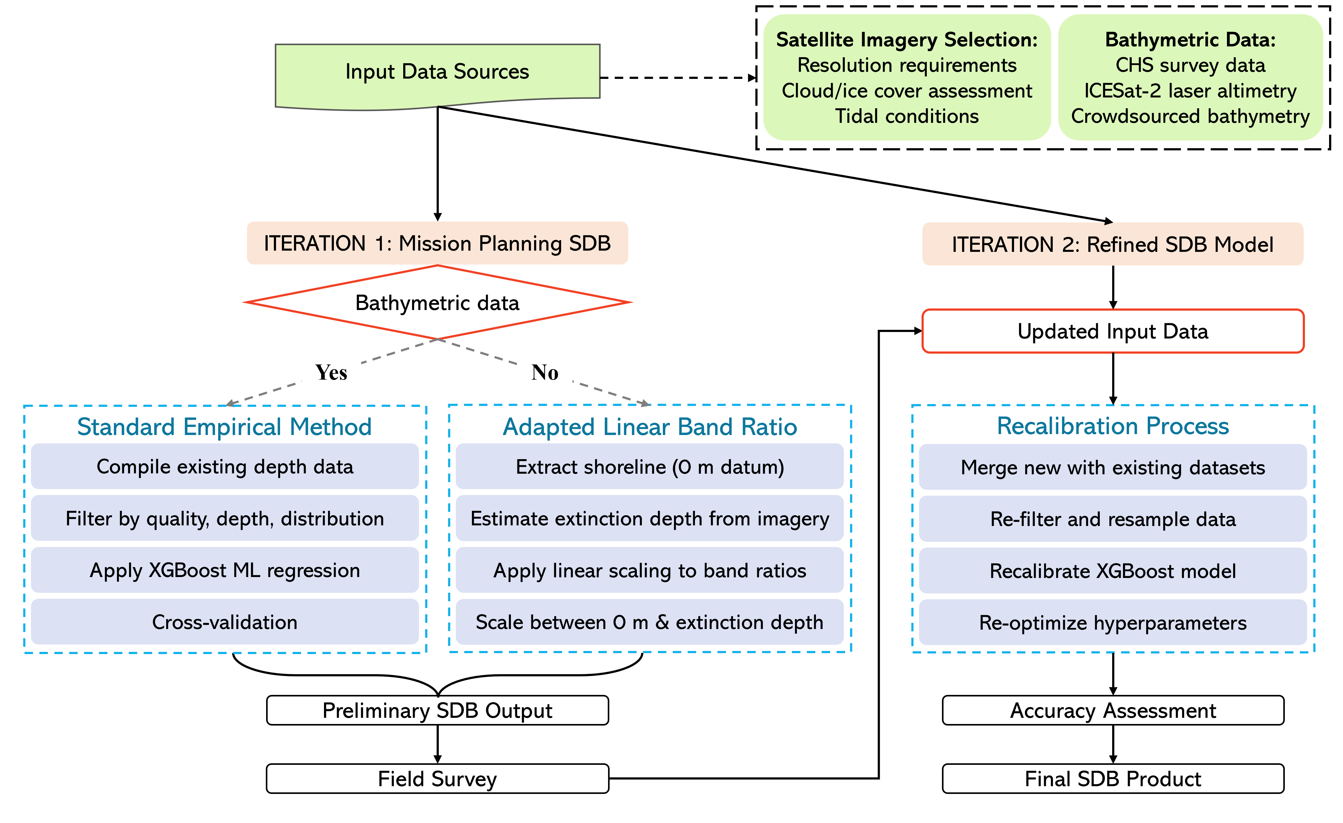
A major limitation in the operational use of empirical SDB is the scarcity of in situ data required both to train the models and to validate the resulting depth estimates. This challenge is particularly relevant for the CHS, as SDB is typically employed to address critical data gaps, precisely in regions where the CHS has little or no existing survey data. For empirical SDB approaches, reference data are essential for model training and accuracy assessment and for ensuring proper calibration to the chart vertical datum. The RSCoE employs an iterative workflow to develop SDB models, with methodological approaches adapted to the availability of bathymetric data. Initial models are used to support survey mission planning, and data collected during surveys are subsequently used to refine model performance and improve the reliability of the resulting bathymetric products (Fig. 2).

2.1.2 Model refinement

Once the field survey is complete, the newly collected data are used to recalibrate and validate the SDB model, thereby improving its accuracy, reliability, and suitability for hydrographic applications. Following the accuracy assessment of the refined SDB, the RSCoE identifies and extracts the portions of the dataset that would improve the safety of nautical products.

The benefit achieved by this two-step iterative approach varies by site and is strongly influenced by both the quality of the original mission planning SDB and the quality of the survey data collected to generate the refined SDB model. In cases where the first iteration mission planning SDB incorporated high quality data and achieved high accuracy, the added value of further model refinement in Step 2 may be reduced. In contrast, where the initial mission-planning SDB relied on limited or poor-quality input data, the collection of depth information in shallow areas within the AOI can lead to significant model improvement. Irrespective of model accuracy improvement, additional survey data still provide valuable information for SDB validation across a larger spatial extent and thus increases confidence in the final SDB product.

2.2 SDB approaches for sites with and without bathymetric data

The RSCoE must create operational remote sensing derived depth products to support mission planning across both charted and uncharted areas of Canadian waters. In most cases where in situ data is available from surveys or LiDAR, satellite derived bathymetry is produced using the empirical approach. In the cases where no in situ data is available, the RSCoE employs an alternative approach by linearly scaling between the 0 m shore and the extinction depth of light in the image, which is estimated on a site-by-site basis based on comparison of charted depths with satellite imagery.

Empirical modeling is the standard SDB approach employed by the RSCoE. This method combines existing depth data with one or more satellite images to model the relationship between depth and pixel colour and apply the model to areas where there is no in situ data. Depth data collected from CHS surveys, ICESat-2 and CSB are identified around the area of interest and assessed for their suitability. The training/validation split typically allocates about 67 % of the data for training and 33 % for validation. However, this ratio can vary because the data are based on data quality, depth range, depth distribution, and geographic coverage. These filters ensure that the final depth dataset is representative of the area of interest and aligns with the spatial extent of the available imagery. Satellite imagery for each area is selected based on the requirements of the project and the location of the AOI, including image resolution, cloud and ice cover, tidal range and heights, and water clarity. Imagery is clipped to ensure that both the AOI for SDB and the area with survey data are included in the image. All SDB analyses with available in situ survey data used an XGBoost machine learning regression model (Chen & Guestrin, 2016), with spectral bands (red, green, blue, and near-infrared) and band-ratio features derived from the logarithmic ratios of visible bands as predictor variables. Model hyperparameters were optimized through randomized cross-validation.

In the absence of in situ depth values, SDB can still be produced; however, its accuracy cannot be measured and must be assumed to be reduced. As its primary purpose is to provide approximate depth values for survey mission planning rather than precise measurements, it can nevertheless offer valuable guidance. In these situations, an adaptation of the linear band ratio method (Stumpf et al., 2003) is employed. This adaptation uses anchor depth points at 0 m and the approximate extinction depth of light in the water, to linearly scale the log ratio of the blue and green bands. The 0 m points are created by extracting the shoreline from lowest available tide imagery and then adjusting for tide height corresponding to the zero of chart datum (water level at 0 m at the LLWLT). Acquiring imagery exactly at the chart datum is often difficult and obtaining a perfect zero‑line snapshot is not always feasible. However, with the wide range of available satellite sources, it is usually possible to obtain images taken within a few centimeters of the lowest water line. For example, Planet’s PlanetScope constellation, comprising of 180 satellites, increases the likelihood of capturing imagery remarkably close to the zero line. Maximum observable depth, defined as the depth at which the seabed remains visible in satellite imagery, is estimated by referencing nearby locations with known depths acquired under comparable conditions (e.g., charted depths from same-date imagery). This estimate is based on visual seabed detectability and may vary spatially with turbidity and bottom reflectance.

The performance of the empirical SDB techniques is calculated by comparing the predicted depth value from the model with coincident in situ depth from survey points in the test dataset and calculating the mean error/bias, the root mean squared error (RMSE), and the 95^th percentile of the absolute error. These metrics were selected to provide a well-rounded assessment of the model performance, including at sites with non- normal error distributions. It is important to note that because the empirical approach for SDB uses in situ data to both train and test for accuracy assessment, the confidence in the results is impacted by the quality of the input data. The use of high-quality survey data collected from official sources can mitigate this concern, but in areas where there are limited data options (e.g. CSB, satellite altimeters) a high accuracy score only indicates high accordance with the in-situ data. Depending on the data quality, this may or may not translate to trustworthy output SDB. In the case of the iterative approach in areas with no bathymetric data for the original SDB, accuracy is expected to be low when compared with newly collected data as the error distribution can be non-normal and incorrect model assumptions can bias the error.

2.3 Case studies

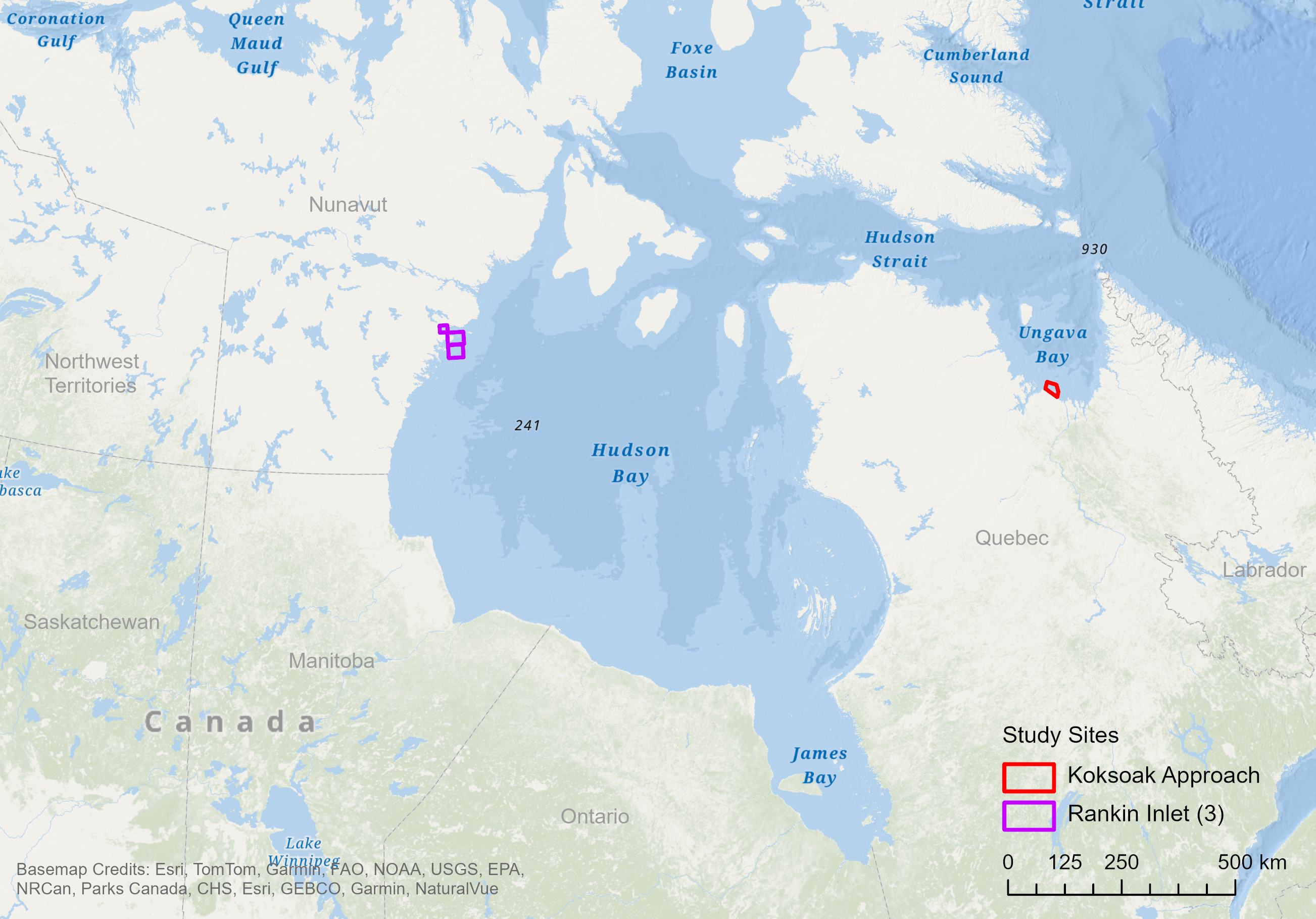
The approaches used to create operational SDB always need to be tailored to a range of factors, such as in situ data availability, imagery quality, and site characteristics. To demonstrate the iterative SDB process employed by the CHS RSCoE, two study sites were selected: (1) the Koksoak Approach, a northern region of Quebec near Kuujjuaq in Ungava Bay, where in situ data were lacking; and (2) Rankin Inlet, Nunavut, where in situ data were available close to the area of interest, which comprises three distinct sub-areas (Fig. 3).

2.3.1 Koksoak Approach

Site and imagery

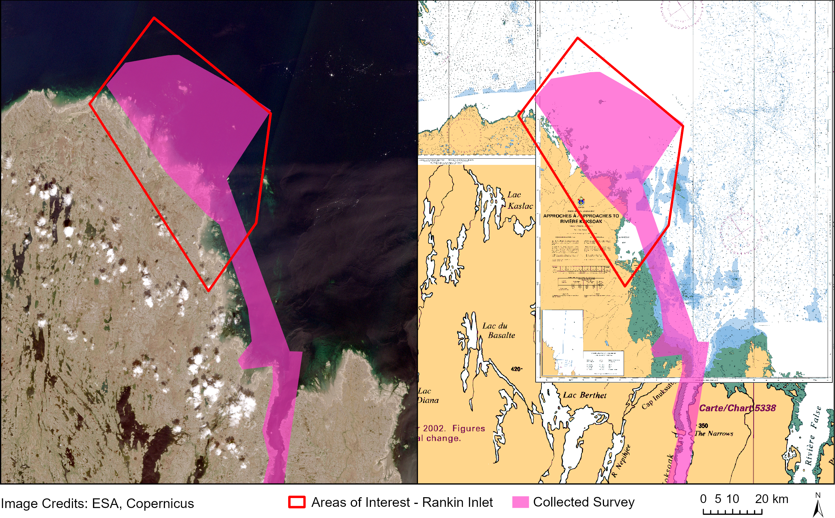
Koksoak Approach is located within the extent of CHS Paper Charts 5300, 5467, and 5376 but is directly in chart “whitespace”, where there are no soundings or other depth information (Fig. 4). Fig. 4 shows the area of interest for initial mission planning SDB (red) and the extent of in situ collected survey (pink) against the Sentinel-2 image (left) and the CHS charts for the area (right). A Sentinel-2 L2A image from 2023-06-29 (3.6 m tide) was used for both the initial SDB for survey mission planning and the second iteration SDB using the newly collected survey data. The tidal range in this area is extremely high (approximately 10 m), and the 3.6 m tide image represents the lowest tide image suitable for SDB, with clear water and no obstruction from cloud or ice.

Bathymetric data and applied methodology

The first iteration of the SDB to support the survey mission was done without in situ data to calibrate a model. The area of interest has no bathymetric information, and the survey data that exist outside of the AOI were unsuitable for model calibration due to insufficient high-quality data at shallow depths within the extent of the Sentinel-2 tile. Instead, the adapted linear band ratio method was used. The 0 m points were created along the land/water boundary of the Sentinel-2 image and then adjusted for tide height. The extinction depth of light in the area was estimated at 13 m based on a comparison of the limited nearby survey data with the satellite image.

The second iteration of the SDB leveraged the CSB survey data collected by the Community Hydrography Program (DFO, 2026) (pink area in Fig. 4) to run an empirical SDB model. The collected CSB data were filtered to depths less than 13 m. Due to the large tidal range in this area, and the path of the survey vessel, the majority of survey data were collected in the intertidal zone (depths above 0 m when adjusted to chart datum LLWLT), leading to a depth range of 5 m above chart datum to 13 m. The dataset was split 67:33 for training and testing, with 63,400 and 27,172 points, respectively. Although spatial autocorrelation may inflate apparent performance metrics, the same data-splitting strategy was applied consistently across all iterations to ensure relative comparability among models.

2.3.2 Rankin Inlet

Site and imagery

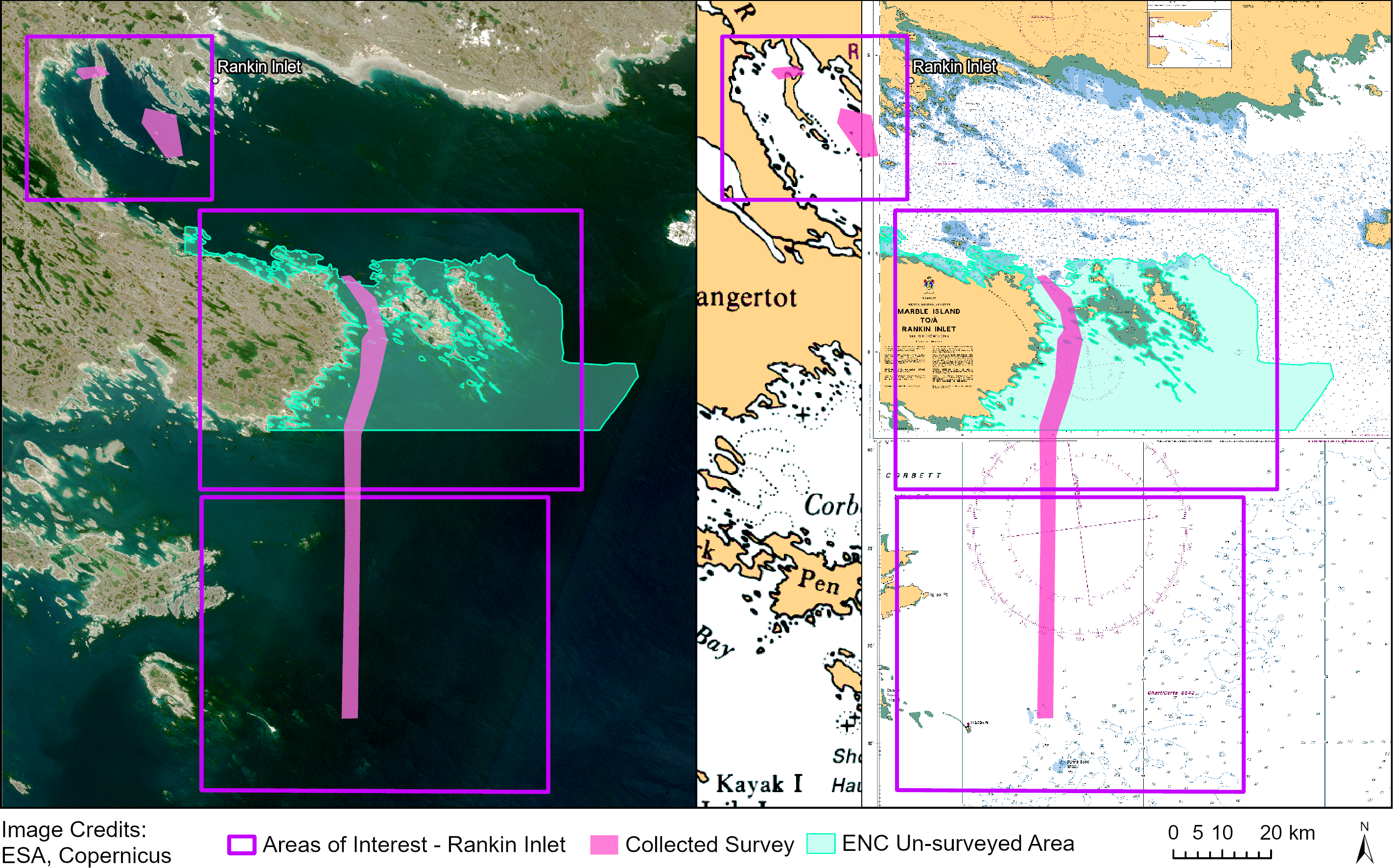
The Rankin Inlet site is split into three AOIs that intersect with parts of CHS Charts 5449, 5630, and 5629 (Fig. 5). The three AOIs correspond to different areas of chart whitespace, where there is no bathymetric information. The original mission planning AOI covered only the central area that corresponds to the unsurveyed region from chart 5630 (shown in turquoise in Fig. 5). The second iteration of the SDB covered a larger area, incorporating all available bathymetric data and extending the coverage to three AOIs (shown in purple in Fig. 5).

Both the first and second iteration SDB derived products used Sentinel-2 L1C imagery from 2018-07-15. For the initial mission planning SDB with a smaller AOI, a single tile 15VWK was used. For the final SDB covering the expanded 3 AOIs, a same-date mosaic covering Sentinel tiles 15VWK and 15VWJ was generated.

In both cases, comparison of the results with the L2A surface reflectance product and the L1C top-of-atmosphere product demonstrated that the L1C imagery yielded slightly higher accuracy, due to reduced performance of the Sen2Cor atmospheric correction over coastal waters in L2A products (Warren et al., 2019).

Bathymetric data and applied methodology

The first SDB iteration supporting mission planning in the Rankin Inlet area used all available CHS multibeam survey data from shallow depths (<15 m). These data were located entirely north of the AOI and did not spatially overlap with it. Of the survey points shallower than 15 m, 87 % were derived from surveys with CATZOC A1 classification and 13 % from surveys classified as CATZOC B. The depth distribution of survey points was strongly right skewed, biasing the dataset toward deeper water. To reduce this bias and improve model performance at shallow depths, the survey points were resampled to approximate a more uniform depth distribution. The filtered dataset was then split into training and testing subsets at a 67:33 ratio, comprising 81,673 and 40,227 points, respectively.

The second iteration of SDB in Rankin Inlet combined the original mission planning dataset with the newly collected CSB data (shown in pink in Fig. 5). Although the CSB data increased the total number of depth points by only 0.06 % (approximately 10,000 points), they improved spatial coverage by providing depth measurements directly within the AOI rather than being confined to areas north of Rankin Inlet. The original CHS training and testing splits were retained, while the CSB data were partitioned using the same 67:33 train test ratio (2,587 training and 5,250 testing points) and subsequently merged with the existing datasets.

3 Results

3.1 Koksoak Approach

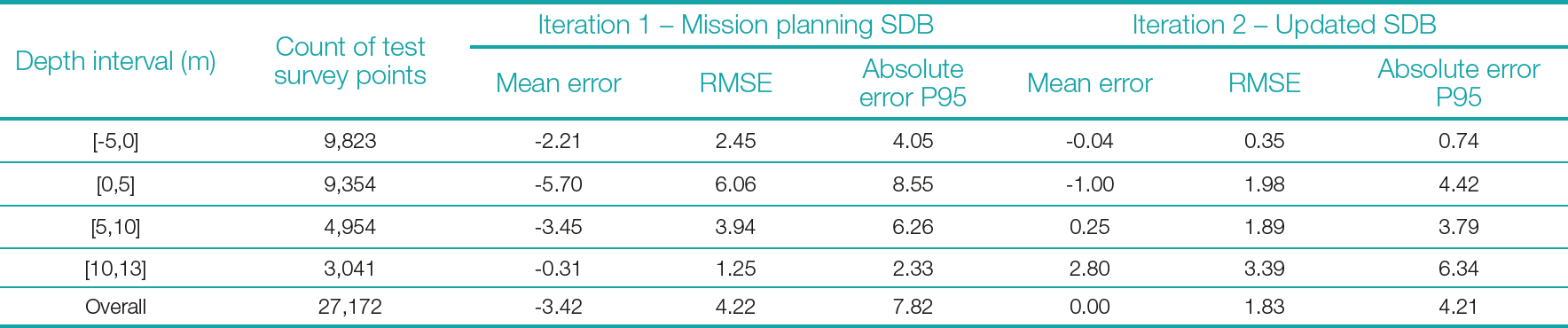
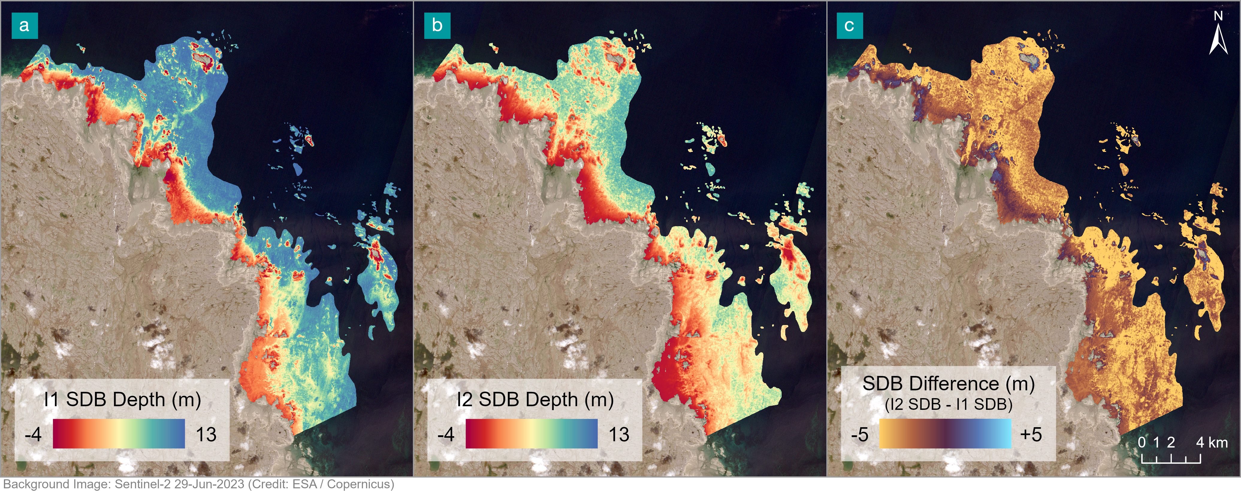
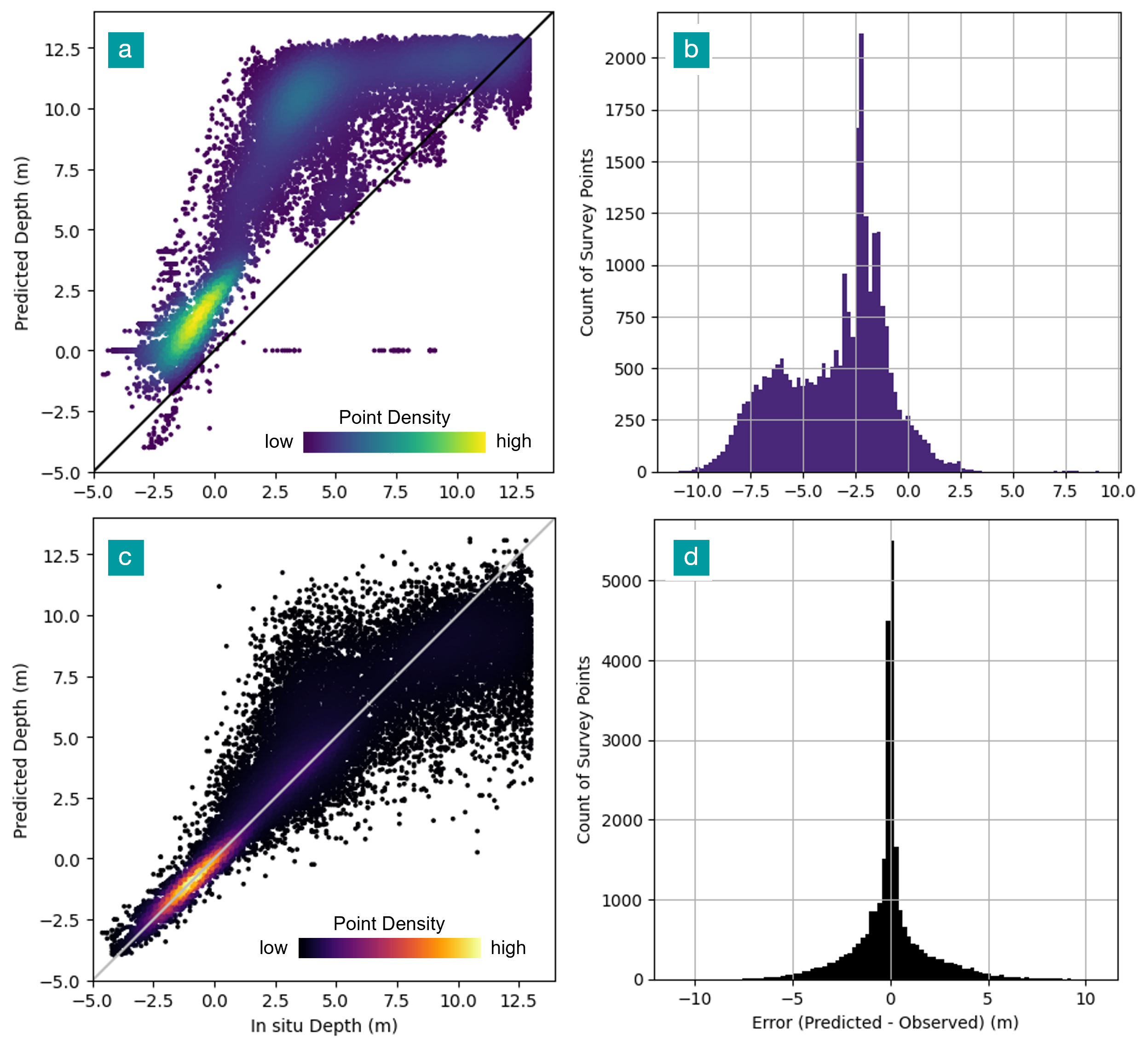
The initial mission planning SDB was produced without an accuracy score because of the absence of in situ data for validation. Its accuracy was evaluated post-mission, once CSB in situ data became available, yielding a mean error of -3.42 m, an RMSE of 4.22 m and 95^th percentile of the absolute error of 7.82 m. The resulting surface is shown in Fig. 6a. Table 1 gives an overview of SDB accuracy by depth. The final SDB model was a machine learning model which achieved a mean error of 0, an overall RMSE of 1.8 m, and the 95^th percentile of the absolute error of 4.21 m. The resulting surfaces and a direct comparison of the two iterations are shown in Fig. 6. Table 1 provides an overview of SDB accuracy by depth interval for both SDB iterations. Fig. 7 presents the comparison between in situ and predicted depth for each data point and the histogram distribution of error for all the survey points that overlapped the SDB achieved a mean error of 0, an overall RMSE of 1.8 m and the 95^th percentile of the absolute error of 4.21 m.

The initial mission planning SDB error showed a strong bias toward overestimation, with predicted SDB depths consistently deeper than observed values. The error distribution was bimodal, with a primary peak around -2 m and a secondary, smaller peak around -6 m (Fig. 7b). Table 1 summarizes error statistics by depth interval, highlighting the same error patterns observed in Fig. 6a. Fig. 7a demonstrates that the original mission planning SDB systematically overestimated depth, particularly in the mid-depth range, but was broadly concordant with the CSB measurements. The bias and high error can be attributed to two things: an incorrect assumption on the extinction depth of light in this area, and complex benthic environment that could not be linearly correlated with pixel brightness. Comparison of the newly collected data within the imagery suggests that the maximum depth in this area varies between 5 m and 10 m below chart datum, for a full range of 9-14 m of water in the selected image (tide of 3.6 m), rather than the 17m initially estimated. The influence of non-uniform benthic environment is shown in Fig. 8, where the first iteration SDB model correlated vegetative substrate with deep water, while the second iteration model better predicted the area as shallow. Although imperfect, the resulting first iteration surface provided valuable supplementary information that enhanced the safety of survey operations by improving situational awareness for mariners collecting new data.

The results were clearly improved for the site when the addition of newly collected data allowed for empirical SDB modeling at the site. The second iteration of SDB modeling at the site demonstrated significant improvement in SDB performance when using CSB data (Fig. 7c and d). However, despite the reduced RMSE, the significant spread of error at depths exceeding 0 m (Fig. 7c) indicates that the second iteration SDB is still of insufficient quality for direct charting applications.

Table 1 shows significantly decreased RMSE outside of the intertidal zone (depths > 0 m), however the RMSE did not decrease monotonically with depth; accuracy improved near 6 m before decreasing again around 10 m. This pattern is also evident in Fig. 7c, where the predicted error starts to be underestimated around 10 m, and in Fig. 6b, where deeper areas were represented by intermediate values (~10 m) rather than the expected maximum depths (~13 m). This behaviour reiterates the limitation in depth retrieval near 10 m, with an effective optical extinction depth of approximately 14 m, given that the survey data depth range began at 4 m above chart datum.

Fig. 6c illustrates the magnitude and spatial distribution of the change between the two SDB surfaces. The updated model produced predominantly shallower depths across most of the AOI (shown in orange), consistent with the reduction in depth overestimation observed when comparing Figs. 7a and 7c. Areas closer to shore exhibited smaller magnitude depth reductions, reflected by darker orange tones in Fig 6c.

For both the mission planning SDB and the updated SDB, complex benthic environments likely contributed to the broad error distributions, as observed in the widely dispersed shapes of the scatter plots and error histograms (Figs. 7a and c). Variability in substrate reflectance, such as dark shallow substrates and bright deeper substrates, can contribute to model uncertainty even where sufficient training data are available, due to limited spectral variance across benthic types.

3.2 Rankin Inlet

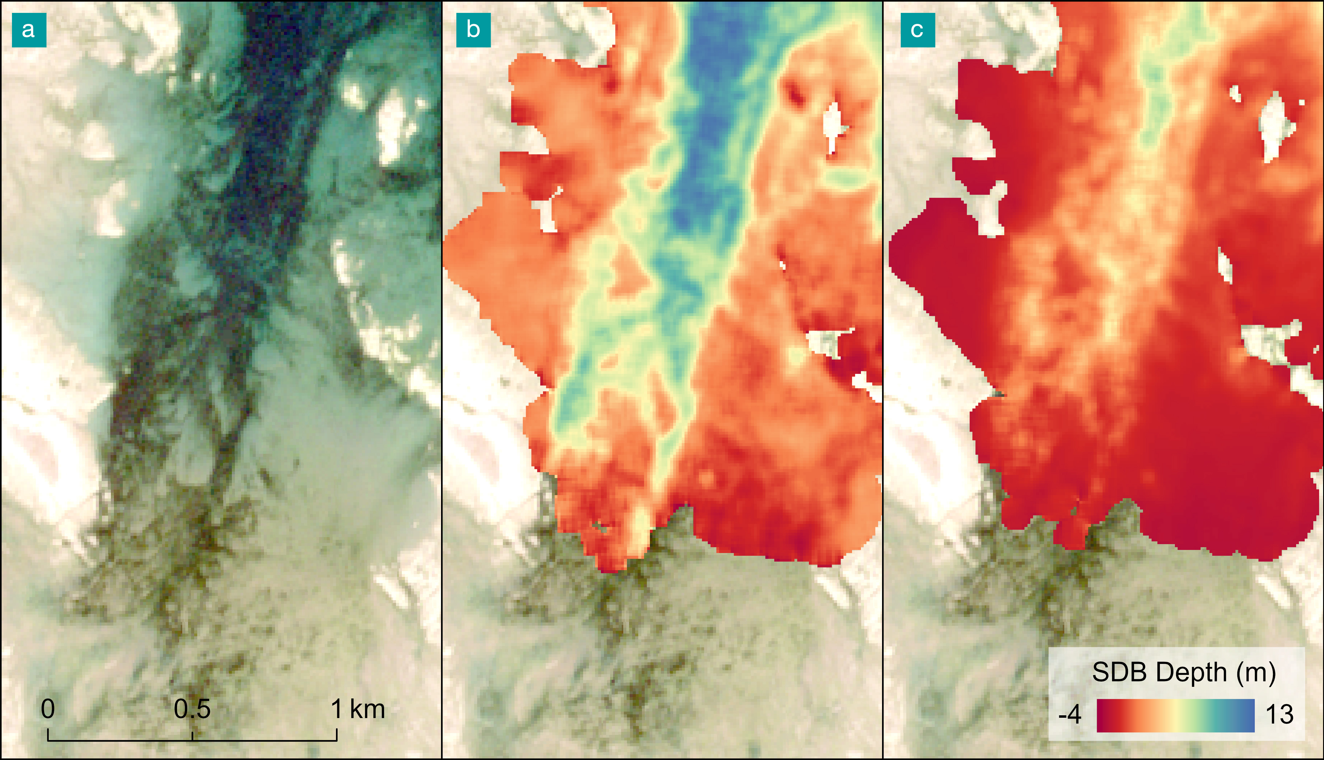
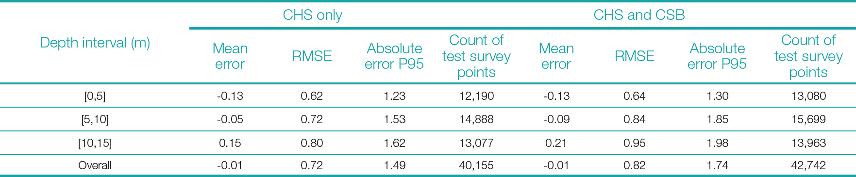
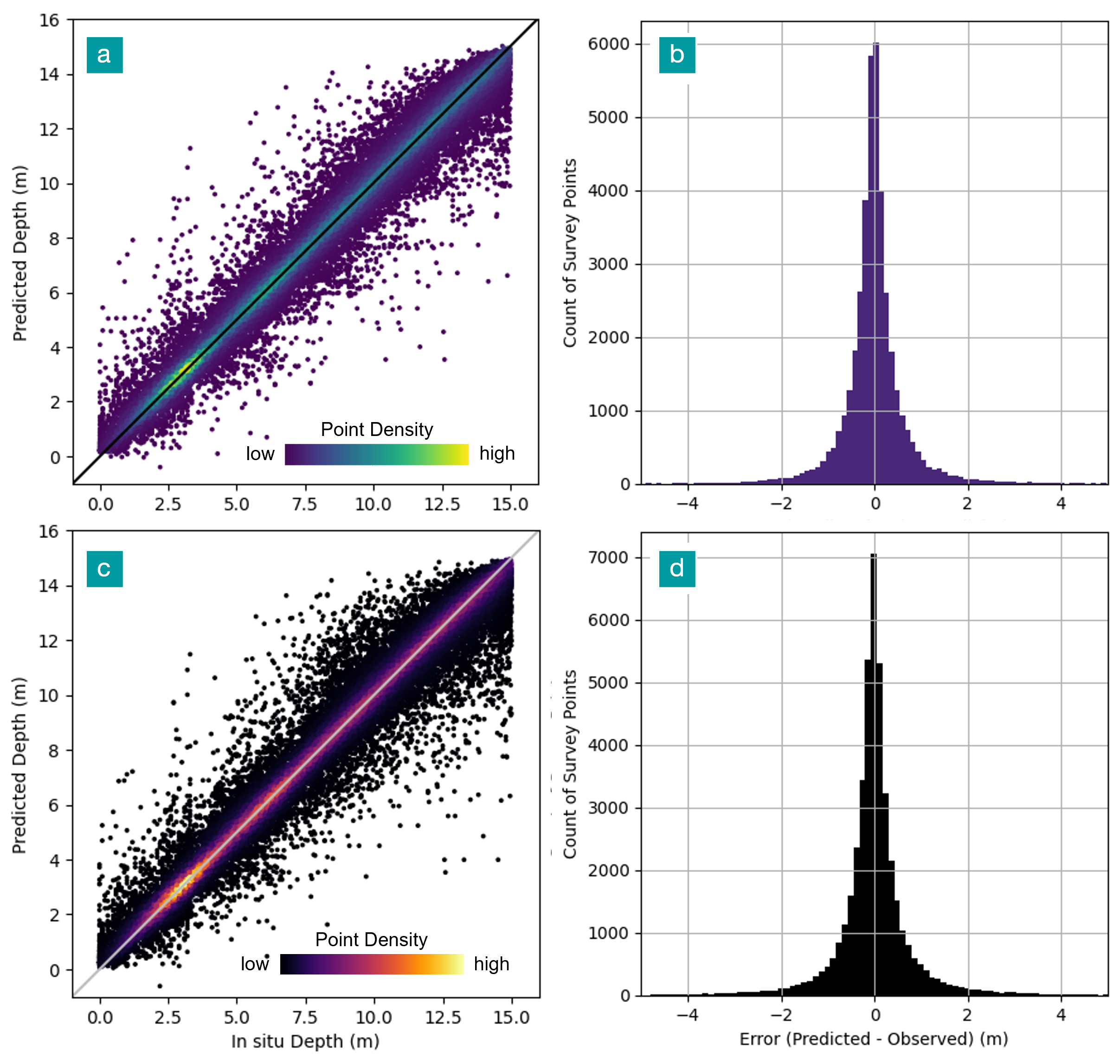
The original mission planning SDB for Rankin Inlet exhibited high accuracy, with a mean error of -0.01, an overall RMSE of 0.72 m and the 95^th percentile of the absolute error of 1.49 m. The final SDB surface for the three AOIs (Fig. 5) is shown in Fig. 9. RMSE decreased slightly with increasing depth but remained low across the full 0–15 m depth range (Table 2). The error distribution shown in Figs. 10a and b indicates strong model performance, with most survey points aligned with the 1:1 line.

The updated SDB model incorporating the newly collected survey points produced no substantial change in overall accuracy, with an updated mean error of -0.01, overall RMSE of 0.82 m and the 95^th percentile of the absolute error of 1.74 m. The resulting surface is shown in Fig. 9b and the difference between the original and updated surfaces is shown in Fig. 9c. Table 2 summarizes model accuracy by depth interval before and after the inclusion of CSB data, demonstrating a consistent and minor increase in RMSE across depth intervals, resulting in an overall increase of approximately 0.1 m. The error distribution (Figs. 10c and 10d) demonstrates minimal difference between the two models, with only a slight increase in the spread of points in Fig. 10c. This limited change is consistent with Fig. 9 which indicates only minor differences between the two surfaces with no distinct pattern, mostly attributable to noise. The exception to this is in the southernmost AOI where the updated SDB appears more sensitive to the image seamline, likely because the additional survey data in this area was collected solely on the eastern side of the image divide (Figs. 5 and 9i).

The minor increase in error likely resulted from the expanded spatial extent of the training data, which introduced greater variability in pixel spectral values and depth, thus increasing the potential for error. Despite this increase, the broader spatial representation improves the applicability of the model across the AOI and increases confidence in the SDB surface over the expanded area.

4 Discussion

4.1 Iterative approach

Analysis of the two study sites showed that the iterative approach was particularly effective in areas where in situ data were sparse, while providing limited additional benefit in areas with extensive existing survey coverage. In both cases, the first SDB iteration provided valuable safety to navigation information that supported crew safety during data collection and helped identify areas where additional surveys would most improve SDB modelling. Results from Rankin Inlet demonstrated that acceptable SDB results can be achieved in the initial iteration, provided that the available in situ data were sufficient in both quantity and quality. Although the addition of CSB data in the second iteration slightly increased global error metrics, the inclusion of in situ data from previously unsurveyed areas increased overall confidence in the application of SDB across the larger AOI.

In contrast, the iterative approach produced substantial improvements in the Koksoak Approach region, which initially lacked adequate in situ data, including shallow water surveys across diverse substrates. At this site, the iterative process enabled the development of a markedly improved SDB model that could be used to derive enhanced hydrographic data for updating nautical products.

While SDB offers significant advantages in data-sparse regions, it also presents unique challenges related to its accuracy and uncertainty assessment. Integrating SDB into hydrographic products requires a clear understanding of its quality characteristics, which can be influenced by factors not typically faced by traditional survey methods, including the methodological approaches, the quality of the input data (both survey measurements and imagery), and site-specific environmental conditions (e.g., sediment type, complex benthic environments). Because SDB represents a modeled depth surface, its accuracy cannot be characterized in the same manner as true in situ survey data. To support the responsible use of SDB in nautical products, it is therefore necessary to clearly define, assess, and communicate SDB quality. The following section distinguishes between system precision, reported accuracy, and product uncertainty, and discusses their implications for nautical charting and related hydrographic applications. Establishing this framework provides a consistent basis for evaluating SDB outputs and supports their appropriate use in updating nautical products.

4.2 Accuracy assessment: precision, accuracy, product uncertainty

In this study, precision refers to system repeatability; accuracy denotes statistical agreement with reference in situ depth measurements, and uncertainty as the spatially varying confidence across the SDB surface (ISO, 2008). A key challenge in SDB and its evaluation is that, unlike traditional survey techniques, such as multibeam echosounders (MBES), single beam echosounders (SBES), or LiDAR, SDB lacks a predefined precision or quantified system of confidence. In contrast to SDB, engineered surveying systems are defined by established performance specifications that characterize system precision and expected accuracy prior to deployment, typically in the decimeter range for MBES (Ernstsen et al., 2006) and LiDAR (Pan et al., 2015) systems in shallow water. This distinction is critical when assessing SDB uncertainty. Although accuracy can be evaluated through validation against in situ measurements, the absence of a defined precision prevents reliable quantification of measurement repeatability under identical conditions (Taylor, 1997). Nevertheless, the application of a consistent and systematic processing workflow can enhance output stability and support a limited degree of repeatability in derived products.

The accuracy assessment is based on a statistical analysis of the differences between a source of water depth – preferably in situ depth measurements and corresponding SDB estimates. Empirical SDB methods rely on the Beer–Lambert Law, which describes the exponential attenuation of light within an absorbing medium, resulting in decreasing water-leaving radiance with increasing depth (Mobley, 1994). Although additional factors influence performance and accuracy, this physical relationship establishes an inherent depth-dependent limitation, with accuracy generally decreasing as water depth increases (Chénier et al., 2018; Duan et al., 2022; Knudby & Richardson, 2023). Consequently, depth-stratified accuracy evaluation is essential to identify the depth ranges over which SDB provides reliable estimates and to delineate outputs suitable for retention or exclusion. In Canadian waters, SDB typically does not exceed depths of about 15 m, and in some regions the effective range is limited to only a few meters. In certain environments, SDB may be impractical altogether due to insufficient light penetration or site complexity that precludes a stable relationship between depth and spectral response.

The principal limitation in characterizing uncertainty in SDB is the lack of sufficient information to assess product quality across the full range of values. This limitation, combined with the lack of well-defined system precision, limits the ability to robustly quantify SDB uncertainty and reduces confidence in the resulting datasets. Because accuracy cannot be assessed for every image pixel, some level of uncertainty is inherent in most SDB products. This is especially true in areas where neighboring pixels show steep spectral transitions and high variability, such as the contrast between high albedo white sand and adjacent dark benthic substrates. Although statistical accuracy metrics derived from validation points provide a useful global indicator of SDB performance, they do not describe spatially explicit uncertainty and therefore cannot represent the spatially varying uncertainty required to evaluate compliance with the International Hydrographic Organization (IHO) S-44 total vertical uncertainty (TVU) requirements. As noted by Taylor (1997), measurement uncertainty arises when observations are incomplete or subject to variable influences, underscoring the importance of error analysis for estimating confidence in measurement results. In the context of SDB, this uncertainty is compounded by environmental and scene-dependent factors, including surface waves, sun glint, suspended sediments, and variability in seabed albedo which introduce spectral variation that complicates depth estimation. The accumulation of systemic and random errors from multiple sources further limits the ability to isolate or eliminate individual error contributions (Taylor, 1997). Consequently, SDB uncertainty and confidence may, in most cases, be difficult to quantify and might need to be acknowledged as an inherent constraint of SDB.

The influence of image resolution on SDB accuracy was not examined in this study, as imagery selection was driven primarily by site extent, with 10 m resolution providing a practical balance of coverage cost, and processing time. Previous work by the CHS RSCoE (Ahola et al., 2020) shows that while higher spatial and spectral resolution can improve SDB performance, environmental conditions have a stronger influence on accuracy than sensor type. As such, freely available medium-resolution imagery can support reliable SDB in appropriate conditions.

It is also important to distinguish spatial resolution from horizontal accuracy, as finer resolution does not necessarily imply improved positional accuracy. However, in complex environments, such as areas with heterogeneous seabed types or steep slopes, medium-resolution data may be insufficient to resolve small but navigationally crucial features, such as isolated rocks. In these cases, higher-resolution imagery is used to support hazard detection, with CHS RSCoE applying ~2 m multispectral data for harbour-scale SDB.

4.3 Application of SDB on nautical products

The most significant limitation to direct application of SDB in official nautical products is the absence of a predefined or guaranteed level of precision. As a result, even when acceptable accuracy is achieved (e.g., ~1 m), quantifying uncertainty across the full SDB surface in accordance with IHO S-44 standards remain extremely challenging (IHO, 2022). This limitation is compounded by the typically sparse availability of validation data, which makes it difficult to assign a reliable Category Zone of Confidence (CATZOC). At the two sites examined, only 1.7 % and 0.4 % of SDB-derived depths could be validated using in situ data at Koksoak Approach and Rankin Inlet, respectively. Given this limited validation coverage, together with environmental and methodological factors affecting depth retrieval, robust evaluation of uncertainty across the full SDB surface is impractical. Accordingly, SDB is not considered reliable for direct incorporation into official nautical products. Consistent with this conclusion, Jai (2025) finds that SDB does not meet S-44 requirements for hydrographic survey data and is better suited for reconnaissance applications. For this reason, the CHS RSCoE does not recommend the direct inclusion of raw SDB in nautical products. When acceptable accuracy is obtained, the RSCoE instead produces derived products, such as isobaths, generated through a combination of SDB and image interpretation to reduce noise and exclude areas that may not represent true water depth.

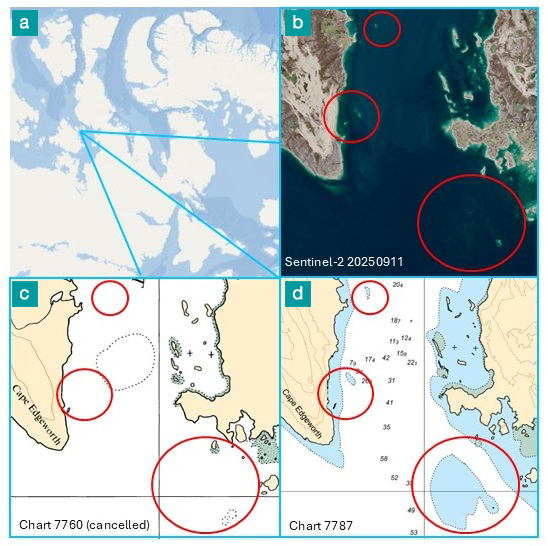
Despite these limitations, SDB remains a valuable resource for enhancing navigation and mission safety. Even at lower accuracy levels, SDB can support meaningful chart improvements. Fig. 11 illustrates a CHS chart that was updated from SDB that was created without any training or validation data. Due to the resulting low confidence in depth estimates, shoal features were charted using the SDB and imagery analysis. The isobaths extracted were charted as areas of unknown depth rather than assigned discrete depth values. This approach improves navigational safety by identifying potentially hazardous shallow areas while avoiding the dissemination of misleading depth information.

The utility of SDB is particularly evident in highly dynamic environments, where rapid sedimentation and erosion can quickly degrade the relevance of existing hydrographic surveys. In such settings, recently acquired SDB has been shown to outperform echosounder data that are only one year old (Chénier et al., 2018). Beyond its accuracy in change prone areas, SDB offers a major advantage for chart timeliness: the frequent revisit cycles of modern satellite missions enable near continuous monitoring of coastal and shallow water zones. This provides hydrographic offices with a cost-efficient means of updating bathymetric information far more regularly than would be feasible with traditional surveys, which can be financially unsustainable to repeat at the frequency required in rapidly evolving environments.

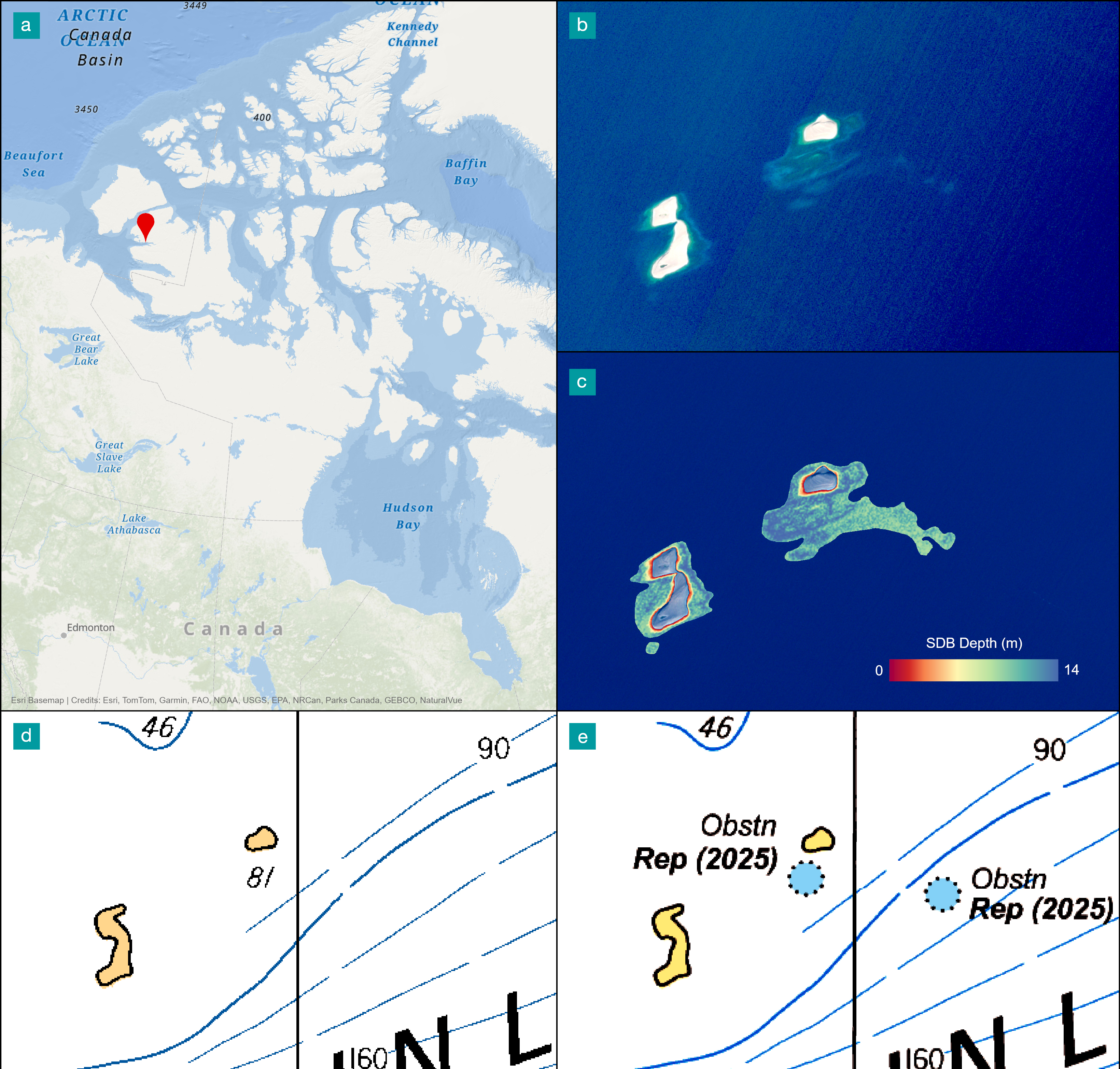
To ensure the safety to navigation for all its projects, the RSCoE systematically analyzes the imagery and the derived remote sensing products to identify potential hazards and obstructions. When preliminary analysis indicates a possible risk, higher-resolution imagery can be obtained to enable a more detailed assessment and confirmation. Features posing immediate risks to navigation may be issued as Navigational Warnings (NAVWARNs; CCG, 2023), while less urgent updates may be disseminated through Notices to Mariners (NOTMARs; CCG, 2025). Collectively, these mechanisms contribute to timely chart updates and the sustained assurance of navigational safety. Fig. 12 presents an example of a navigational hazard identified using remote sensing techniques and subsequently issued as a NAVWARN.

4.4 Future development

While this paper does not compare different SDB approaches, the uncertainty associated with SDB is not method specific. At CHS, SDB models are generated using a range of approaches (empirical, photogrammetric, and physics-based), each with distinct advantages and limitations. However, all are influenced by fundamental constraints related to light penetration through the water column and reflectance from the seafloor. Where the seafloor is not optically detectable, reliable depth estimation is not possible.

Environmental conditions are a primary source of uncertainty across all SDB approaches. Suspended sediments reduce bottom detectability by scattering or absorbing light, while high sediment albedo can cause the dominant reflectance to originate from the water column or surface rather than the seabed, leading to significant depth errors. Conversely, low-reflectance benthic substrates, such as dark vegetation, produce weak or ambiguous signals that also degrade model performance.

Photogrammetry can offer improved performance in some benthic environments due to enhanced textural contrast, which supports image matching and feature detection (Chénier et al., 2019). However, it is not without limitations: it performs best along sharp edges, and derived depths may correspond to the top of benthic vegetation rather than the true seafloor. Although this effect is reduced in Arctic environments where vegetation is typically low-growing, the limitation remains.

To reduce uncertainty in SDB, the CHS has developed a level‑of‑confidence approach (Chénier et al., 2019). This method improves confidence in SDB by comparing several independent SDB datasets and retaining only the depth values that agree within 1 m. This filtering step effectively removes large errors from the final product. For example, at a site in Cambridge Bay, approximately 80 % of the SDB values met the 1 m agreement criterion, leaving only 20 % of the SDB surface requiring further evaluation (Chénier et al., 2019). A major limitation of this approach in operational contexts is the substantial time and resources required to generate multiple independent SDB datasets. Producing several SDB layers, regardless of the underlying method, demands additional data acquisition, processing effort, and computational capacity. For instance, photogrammetric SDB requires stereo imagery, which further increases acquisition and processing requirements. As a result, the approach can become costly and difficult to implement routinely in large‑scale or time‑sensitive environments. It also requires the use of diverse imagery, because not all errors originate from seafloor characteristics. Many issues instead arise from the atmosphere (clouds, haze, shadows), the sea surface (waves, sun glint, suspended sediment, floating aquatic vegetation, and debris), or the water column itself (turbidity, sediment load, light angle, submerged aquatic vegetation). The development of more automated workflows could help reduce the time needed to run the CHS level‑of‑confidence approach and improve not only the accuracy but, more importantly, the reliability of the results.

Another way to improve understanding of error sources and reduce their influence on SDB is to incorporate classification‑based approaches. For example, classification methods can be used to identify and map vegetation that interferes with SDB retrieval. Implementing seabed‑type classification (Chénier et al., 2019) can help highlight areas that are inherently more challenging for depth estimation. In addition, masking vegetation using a Chlorophyll Index has been shown to effectively remove portions of SDB outputs that do not provide reliable depth information (Caballero et al., 2020).

5 Conclusion

The iterative approach developed by the CHS ensures that SDB products effectively support navigational safety and the ongoing modernization of nautical charts when applied within an operational framework. This approach enables the rapid production of preliminary products that support survey planning and enhance crew safety. In areas with limited in situ data, incorporating recent and higher-quality measurements allows SDB models to be refined, resulting in derived products that are better suited for updating nautical products. A limitation of this study is that validation coverage remains spatially sparse relative to total SDB area, which restricts full characterization of spatial uncertainty patterns.

However, because SDB lacks predefined system precision and robust uncertainty quantification, it cannot achieve the accuracy or confidence levels of MBES data. As a result, raw SDB outputs are unsuitable for direct incorporation into official nautical products. Despite advances in automation and artificial intelligence, expert intervention by remote sensing specialists remains essential to ensure reliable and responsible chart updates (Chénier et al., 2024). When appropriately assessed and integrated, remote sensing products can identify navigational hazards, including previously uncharted shoals, thereby reducing risk to mariners. In highly dynamic environments, where traditional surveys rapidly become outdated, SDB provides a valuable complementary tool for maintaining chart relevance and supporting safe navigation. Improving SDB uncertainty and better quantifying accuracy will remain key priorities for CHS, with ongoing efforts aimed at reducing manual intervention. Future development will be made in better integrating image‑classification techniques to identify factors such as benthic environments and sediment that can introduce large errors in SDB. The CHS confidence‑level approach should also be better integrated in an operational context by providing a structured way to quantify reliability and build trust in SDB products. Together, these developments move SDB toward more reliable operational use. Continued refinement of confidence metrics, increased automation in feature classification, and improved sensor‑driven environmental characterization will be essential to reducing uncertainty and expanding SDB’s practical value in hydrographic applications.

Acknowledgements

The authors gratefully acknowledge the support of Sarah-Anne Seale, Adam Jirovec, Chris Hemmingway, and Hamid Jafarzadeh for assistance with figure preparation and manuscript review. We appreciate their valuable feedback.

References

Ahola, R., Chénier, R., Sagram, M. and Horner, B. (2020). The impact of sensors for satellite derived bathymetry within the Canadian Arctic. Geomatica, 74(2), pp. 46–64. https://doi.org/10.1139/GEOMAT-2019-0022

Caballero, I. and Stumpf, R. P. (2020). Towards Routine Mapping of Shallow Bathymetry in Environments with Variable Turbidity: Contribution of Sentinel-2A/B Satellites Mission. Remote Sensing, 12(3). https://doi.org/10.3390/rs12030451

CCG (2023). Navigational and NAVAREA warnings. Canadian Coast Guard, Government of Canada, Canada. https://www.ccg-gcc.gc.ca/mcts-sctm/navwarn-avnav-ca-eng.html (last accessed 21 August 2025).

CCG (2025). Notices to Mariners (NOTMAR). Canadian Coast Guard, Government of Canada, Canada. https://www.notmar.gc.ca/index-en (last accessed 21 August 2025).

Chen, T. and Guestrin, C. (2016). XGBoost: A Scalable Tree Boosting System. Proceedings of the 22nd ACM SIGKDD International Conference on Knowledge Discovery and Data Mining, pp. 785–794. https://doi.org/10.1145/2939672.2939785

Chénier, R., Ahola, R., Sagram, M., Faucher, M.-A. and Shelat, Y. (2019). Consideration of Level of Confidence within Multi-Approach Satellite-Derived Bathymetry. ISPRS International Journal of Geo-Information, 8(1), 48. https://doi.org/10.3390/ijgi8010048

Chénier, R., Faucher, M. A. and Ahola, R. (2018). Satellite-Derived Bathymetry for Improving Canadian Hydrographic Service Charts. ISPRS International Journal of Geo-Information 2018, 7(8), p. 306. https://doi.org/10.3390/IJGI7080306

Chénier, R., Faucher, M.A., Ahola, R., Jiao, X. and Tardif, L. (2016). Remote sensing approach for updating CHS charts. Proceedings of the Canadian Hydrographic Conference, Halifax, Canada.

Chénier, R., Faucher, M.-A., Ahola, R., Shelat, Y. and Sagram, M. (2018). Bathymetric Photogrammetry to Update CHS Charts: Comparing Conventional 3D Manual and Automatic Approaches. ISPRS International Journal of Geo-Information, 7(10), 395. https://doi.org/10.3390/ijgi7100395

Chénier, R., Omari, K. and Seale, S.-A. (2024). Leveraging Earth Observation Data To Enhance The Safety To Navigation In The Canadian Arctic. Proceedings of IEEE International Geoscience and Remote Sensing Symposium (IGARSS), Athens, Greece.

Chénier, R., Omari, K., Blondel, E., Sagram, M. and Jirovec, A. (2020a). Accelerating the Usage of Earth and Oceans Observation Data in Hydrographic Applications. The International Hydrographic Review, 24, pp. 103–127. https://ihr.iho.int/articles/accelerating-the-usage-of-earth-and-oceans-observation-data-in-hydrographic-applications/ (last accessed 22 April 2025).

Chénier, R., Omari, K., George, G., Lounissi, L., Seale, S.-A., Abado, L., and Gautam, S. (2025). Remote sensing technology utilized by CHS to support safety of navigation in the Arctic. Proceedings of Remote Sensing for Agriculture, Ecosystems, and Hydrology XXVII, 13666, pp. 26–40. https://doi.org/10.1117/12.3069938

Chénier, R., Sagram, M., Omari, K. and Jirovec, A. (2020b). Earth Observation and Artificial Intelligence for Improving Safety to Navigation in Canada Low-Impact Shipping Corridors. ISPRS International Journal of Geo-Information, 9(6), 383. https://doi.org/10.3390/ijgi9060383

Dekker A. G., Phinn S. R., Anstee J., Bissett P., Brando V. E., Casey B., Fearns P., Hedley J., Klonowski W., Lee Z. P., Lynch M., Lyons M., Mobley C. and Roelfsema C. (2011). Intercomparison of shallow water bathymetry, hydro-optics, and benthos mapping techniques in Australian and Caribbean coastal environments. Limnol. Oceanogr. Methods, 9. https://doi.org/10.4319/lom.2011.9.396

DFO (2026). Community Hydrography. Department of Fisheries and Oceans, Government of Canada, Canada. https://www.dfo-mpo.gc.ca/science/hydrography-hydrographie/opp-ppo/index-eng.html (last accessed January 21, 2026).

Duan, Z., Chu, S., Cheng, L., Ji, C., Li, M. and Shen, W. (2022). Satellite-derived bathymetry using Landsat-8 and Sentinel-2A images: assessment of atmospheric correction algorithms and depth derivation models in shallow waters. Opt. Express, 30, 3238–3261. https://doi.org/10.1364/OE.444557

Ernstsen, V. B., Noormets, R., Hebbeln, D., Bartholomä, A., and Flemming, B. W. (2006). Precision of high-resolution multibeam echo sounding coupled with high-accuracy positioning in a shallow water coastal environment. Geo-Marine Letters, 26(3), pp. 141–149. https://doi.org/10.1007/s00367-006-0025-3

Hodúl, M., Bird, S., Knudby, A. and Chénier, R. (2018). Satellite derived photogrammetric bathymetry. ISPRS Journal of Photogrammetry and Remote Sensing, 142, pp. 268–277. https://doi.org/10.1016/J.ISPRSJPRS.2018.06.015

IHO (2022). Standards for Hydrographic Surveys (6^th ed.). IHO Special Publication S-44, International Hydrographic Organization, Monaco. https://iho.int/uploads/user/pubs/standards/s-44/S-44_Edition_6.1.0.pdf (last accessed 21 January 2026).

ISO (2008) ISO/IEC Guide 98-3:2008 – Uncertainty of measurement — Part 3: Guide to the expression of uncertainty in measurement (GUM:1995). International Organization for Standardization. https://www.iso.org/standard/50461.html (last accessed 21 January 2026).

Jai, V. (2025). Evaluation of SDB data for near shore mapping around Agatti Island, India: a comparative study with echo sounder survey. The International Hydrographic Review, 31(2). https://doi.org/10.58440/ihr-31-2-n07

Kerr, J. M. and Purkis, S. (2018). An algorithm for optically-deriving water depth from multispectral imagery in coral reef landscapes in the absence of ground-truth data. Remote Sensing of Environment, 210, pp. 307–324. https://doi.org/10.1016/J.RSE.2018.03.024

Knudby, A. (2025). Satellite imagery for hazard detection: better use of satellite imagery could help prevent groundings in the Canadian Arctic. The International Hydrographic Review, 31(2). https://doi.org/10.58440/ihr-31-2-a13

Knudby, A. and Richardson, G. (2023). Incorporation of neighborhood information improves performance of SDB models. Remote Sensing Applications: Society and Environment, 32, p. 101033. https://doi.org/10.1016/J.RSASE.2023.101033

Knudby, A., Ahmad, S. K. and Ilori, C. (2016). The Potential for Landsat-Based Bathymetry in Canada. Canadian Journal of Remote Sensing, 42(4), pp. 367–378. https://doi.org/10.1080/07038992.2016.1177452;CTYPE:STRING:JOURNAL

Lee, Z., Carder, K. L., Mobley, C. D., Steward, R. G.and Patch, J. S. (1999). Hyperspectral remote sensing for shallow waters: 2. Deriving bottom depths and water properties by optimization. Applied Optics, 38(18), pp. 3831–3843, pp. 3831–3843. https://doi.org/10.1364/AO.38.003831

Lyzenga, D. R. (1978). Passive remote sensing techniques for mapping water depth and bottom features. Applied Optics, 17(3), pp. 379–383. https://doi.org/10.1364/AO.17.000379

Lyzenga, D. R. (1981). Remote sensing of bottom reflectance and water attenuation parameters in shallow water using aircraft and Landsat data. International Journal of Remote Sensing, 2(1), 71–82. https://doi.org/10.1080/01431168108948342

Lyzenga, D. R. (1985). Shallow-water bathymetry using combined lidar and passive multispectral scanner data. International Journal of Remote Sensing, 6(1), pp. 115–125. https://doi.org/10.1080/01431168508948428;ISSUE:ISSUE:DOI

Lyzenga, D. R., Malinas, N. P. and Tanis, F. J. (2006). Multispectral bathymetry using a simple physically based algorithm. IEEE Transactions on Geoscience and Remote Sensing, 44(8), 2251–2258. https://doi.org/10.1109/TGRS.2006.872909

Mobley, C. D. (1994). Light and Water: Radiative Transfer in Natural Waters. Academic Press.

Mobley, C. D. (ed.) (2022). The Oceanic Optics Book. International Ocean Colour Coordinating Group (IOCCG), Dartmouth, NS, Canada, 924pp. https://doi.org/10.25607/OBP-1710

Pan, Z., Glennie, C., Hartzell, P., Fernandez-Diaz, J. C., Legleiter, C. and Overstreet, B. (2015). Performance Assessment of High Resolution Airborne Full Waveform LiDAR for Shallow River Bathymetry. Remote Sensing, 7(5), 5133–5159. https://doi.org/10.3390/rs70505133

Polcyn, F. C., Brown, W. L. and Sattinger, I. J. (1970). The Measurement of Water Depth by Remote Sensing Techniques. Report No. 8973-26-F [Preprint]. Ann Arbour, MI, USA: Willow Run Laboratories of the Institute of Science and Technology, the University of Michigan.

Stumpf, R. P., Holderied, K. and Sinclair, M. (2003). Determination of water depth with high-resolution satellite imagery over variable bottom types. Limnology and Oceanography, 48(1part2), pp. 547–556. https://doi.org/10.4319/LO.2003.48.1_PART_2.0547

Taylor, J. R. (1997) An Introduction to Error Analysis: The Study of Uncertainties in Physical Measurements (2^nd ed). University Science Books.

TC (2023). Oceans Protection Plan. Transport Canada, Government of Canada, Canada. https://tc.canada.ca/en/corporate-services/transparency/briefing-documents-transport-canada/2023/current-topics/oceans-protection-plan (last accessed 18 August 2025).

Warren, M. A., Simis, S. G. H., Martinez-Vicente, V., Poser, K., Bresciani, M., Alikas, K., Spyrakos, E., Giardino, C. and Ansper, A. (2019). Assessment of atmospheric correction algorithms for the Sentinel-2A MultiSpectral Imager over coastal and inland waters. Remote Sensing of Environment, 225, pp. 267–289. https://doi.org/10.1016/J.RSE .2019.03.018

Authors’ biographies

René Chénier is a manager at the Canadian Hydrographic Service (CHS), where he oversees the Geodesy, Geomatics, and Remote Sensing groups. Over his 17 years with CHS, he established the organization’s Remote Sensing Centre of Expertise (RSCoE) and has led numerous initiatives advancing marine and coastal mapping capabilities. His expertise includes Satellite‑Derived Bathymetry (SDB), Interferometric Synthetic Aperture Radar (InSAR), polarimetry, geometric modeling, photogrammetry, digital elevation modeling, and AI‑based image classification. His work also spans ship detection and monitoring, hydrography, cartography, coastal erosion assessment, and habitat mapping.

Genevieve George is a remote sensing professional working with the Remote Sensing Centre of Expertise at the Canadian Hydrographic Service (CHS). Her work at the CHS focuses primarily on operational satellite derived bathymetry. She has broad expertise in imagery analysis across multiple sensor types and applications, with a particular emphasis on applying machine learning techniques to extract, model, and interpret geospatial data.

Loretta Abado has worked with the Canadian Hydrographic Service (CHS) since 2014 within the Remote Sensing Centre of Expertise (RSCoE). Her work focuses on the application of geomatics and remote sensing to support hydrographic operations. She contributes to the development and operationalization of remote sensing workflows that support safe navigation.

Khalid Omari received the Ph.D. and M.Sc. degrees in remote sensing from the Ottawa–Carleton Geoscience Centre, University of Ottawa, Canada, in 2009 and 2002, respectively. He worked for 14 years as a Remote Sensing Scientist at the Canada Centre for Remote Sensing (CCRS), Natural Resources Canada, later part of the Canada Centre for Mapping and Earth Observation (CCMEO). He is currently a Remote Sensing Scientist with the Canadian Hydrographic Service (CHS), Fisheries and Oceans Canada (DFO), where he develops and applies Earth observation–based methodologies and products for hydrographic applications. His research interests include SAR polarimetry and interferometry, as well as optical multispectral and hyperspectral remote sensing. His doctoral research focused on radiative transfer modeling in vegetation canopies and retrieval of biophysical and biochemical parameters from hyperspectral data.