1 Introduction

The hydrographic survey ships use positioning and orientation systems (POS) in conjunction with sonar systems to determine seafloor positions and depths. Modern surface POS consists of two subsystems: a global navigation satellite system (GNSS) unit with two antennas and an inertial measurement unit (IMU) (Kongsberg, 2024; SBG, 2025; Applanix, 2025). On the multibeam side, high-frequency, shallow water sonars may have transmit and receive arrays mounted on machined frames and generally enclosed in a single casing, while low-frequency sonars (e.g., 100 kHz or lower, such as EM 304 (Kongsberg, 2021), SeaBeam 3050 (ELAC Sonar, 2021), and HydroSweep DS (Teledyne Marine, 2022)) have separate transmit (Tx) and receiver (Rx) arrays mounted on the ship. To integrate these systems properly, it is crucial to understand the spatial and angular relationship of all physical components, including GNSS antennas, IMU, multibeam Tx and Rx arrays, with respect to a common reference frame, typically referred to as the vessel reference frame (VRF).

A coordinate reference system (CRS) defines the rules for measuring coordinates within a specific framework (Vaníček & Krakiwsky, 2015). In the context of a vessel reference system, these rules include defining:

1. the location of the origin of the coordinate system, which can be a physical or virtual point on the vessel (e.g., a center of gravity, IMU reference mark or phase center, sonar acoustic center, or a granite reference block (IMTEC Group, 2021; Westlake Consultant, 2021)) or a fictitious point anywhere in or outside the vessel (Hiroji & Oderinde, 2022);
2. the orientation of three orthogonal axes, which typically follows the POS or sonar coordinate system’s convention;
3. the linear scale, which is one for VOS given the small distances involved (a few hundred meters); and
4. the unit of measure, which is usually consistent with the hydrographic data collection software.
   The VRF is the physical realization of the vessel’s

The VRF is the physical realization of the vessel’s CRS, requiring the identification of specific points on the vessel relative to the defined origin and orientation of axes. Establishing the VRF is one of the objectives of any VOS, followed by measuring the spatial and angular offsets of onboard systems relative to the realized VRF. VOS are referred to by various terms, including Dimensional Control Survey, Alignment Survey, Vessel Configuration Survey, or Vessel Geometry Survey. In some cases, they are even called Land Surveys as these surveys are often conducted on land in a dry dock. These different names reflect the same underlying objective: to precisely measure and define the spatial and angular relationships of various system components to ensure accurate integration and performance of the hydrographic and positioning systems.

1.1 Accuracy requirement of VOS

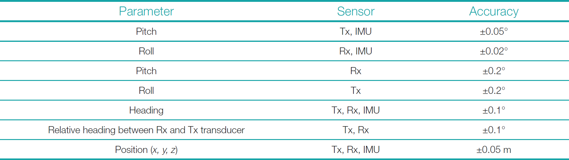
The deviations of spatial and angular offsets of various system components critically influence system performance (Applanix, 2017; Kongsberg, 2021). For instance, any error in the spatial relationship of GNSS antennas directly impacts the accuracy of position and heading. Similarly, any error in the IMU’s angular alignment with the VRF directly affects the orientation accuracy. Given the three-dimensional spatial relationships among system components and the three degrees of freedom in orientation, errors in spatial and angular offsets measured during VOS introduce non-linear effects on final bathymetry (Hughes Clarke, 2003). In general, larger spatial offsets between system components and increased vessel motion exacerbate the impact of errors in VOS on the position and motion outputs from POS, multibeam and other system performance, ultimately affecting the accuracy of seafloor position and depths. In some cases, the manufacturers of hydrographic systems provide the minimum accuracy with which various offsets must be obtained during VOS. An example of such a requirement is shown in Table 1.

In all multibeam systems with separate Tx and Rx arrays, the angular relationship between Tx and Rx is crucial to sonar performance (90° ± 2°). The most stringent linear accuracy requirement during VOS is for the flatness of different modules of the Tx and Rx units; for example, for Kongsberg systems, this is 0.6 mm (Kongsberg, 2021). Similarly, the most stringent angular requirement can be for Applanix POS MV Ocean Master IMU at ±0.008° at its highest performance level (Applanix, 2017).

1.2 Patch test and VOS

Before delving into the experiments and analysis, it is essential to clarify why a multibeam patch test cannot replace VOS. When the first multibeam systems were deployed, it was found that residual angular offsets, the remaining angular offset after applying offsets computed during VOS, and latency between positioning and sonar system could introduce significant systematic errors in seafloor positioning (Hughes Clarke, 2018). To address this, a field calibration process, commonly known as the multibeam patch test, was developed to estimate these residual angular offsets. The patch test, now a standard procedure following new sonar installations, derives residual roll and pitch offsets between the IMU and the multibeam system (combined Tx and Rx), along with the residual heading offset between the heading device and the multibeam system (combined Tx and Rx). The patch test results are applied in addition to the angular offsets obtained from VOS. Typically, a patch test provides roll offsets with an angular resolution on the order of 0.001° and pitch and yaw offsets on the order of 0.01°, as demonstrated in published technical reports from the U.S. academic research fleet (MAC, 2024).

However, the patch test estimates only the residual angular offsets and does not replace the need for the initial angular and spatial offsets derived through VOS. The patch test provides three residual angular misalignments: roll, pitch, and yaw. However, it is important to acknowledge the limitations of the patch test. First, it cannot estimate the angular misalignment between a system’s reference frame and the VRF. The patch test only addresses the residual misalignment between the sonar and other systems (Hughes Clarke, 2003). For instance, if an IMU has a roll mounting angular error of -0.05° with VRF and the combined transmit (Tx) and receive (Rx) multibeam system has a mounting angle error of +0.05° with VRF, the patch test will theoretically show a residual roll offset with a magnitude of 0.10° to be applied to the IMU or Tx and Rx, with the sign depending on the adopted coordinate-system convention and the correction definition.

Additionally, the patch test cannot detect the angular misalignment between the separate multibeam Tx and Rx units in low-frequency sonar systems. Residual errors in this alignment remain undetectable, but significant unaccounted misalignment degrades the performance of the sonar system, especially in the mathematical beamforming process where the Tx and Rx cone intersections are computed.

Moreover, the patch test does not account for the heading misalignment between the IMU forward axis and the VRF forward axis. Since the heading in the POS system is primarily derived from the GNSS vector, the residual heading value from the patch test does not reflect the IMU’s heading misalignment with the VRF. Any misalignment left uncorrected will distort the IMU’s roll and pitch readings, with the error increasing in magnitude as higher roll and pitch motion are experienced.

Because of the above reasons, while the patch test can reduce systematic errors in bathymetric data, it cannot fully eliminate the effects of residual angular misalignments and their cross-talk. The only way to minimize these errors effectively is through a high-accuracy VOS.

1.3 Motivation for this study

Typically, a sonar manufacturer or a shipyard contracts a survey company to conduct a VOS. The survey company is usually provided with the minimum requirements set by the equipment manufacturers. The resulting reports detail the computed offsets, aiming to present the information in a user-friendly format and to prevent misunderstandings in sign conventions. In some cases, a national advisory committee provides guidelines for standardizing these reports across different survey companies and vessels for a national fleet (MAC, 2024). However, a review of several reports, along with discussions with survey companies and contractors, reveals that while minimum accuracy requirements and report guidelines are provided, there are no publicly available formal standards or guidelines outlining how the survey itself should be designed and executed. In addition, IHO S-44 (IHO, 2022) does not provide specific guidance on minimum accuracy or uncertainty requirements for vessel offset surveys, either in general or by survey order. We hope that this study represents a step toward the development of a more standardized, traceable, and technically defensible approach for conducting VOS.

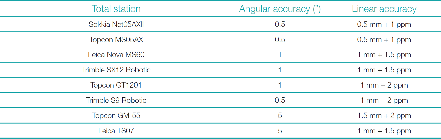
The methodology for performing a VOS is typically left to the discretion of the surveyors and is not required to be detailed in the final report. In the absence of standardized procedures, key variables, such as the accuracy of the instrumentation, the number of redundant observations, the methods for computing angular offsets, and the overall observed uncertainties, can vary significantly between survey companies. A review of recent VOS reports for the U.S. academic fleet (IMTEC Group, 2021) indicates that general estimates for both linear and angular accuracies are provided. Linear accuracies are typically reported between 1 mm to 2 mm, which is generally twice the distance measurement accuracy of the instrument used. Angular accuracies are reported between 30” and 60”, corresponding to approximately 60 times the angular accuracies of the instrument used. Mostly, the instrument used for VOS is a total station, an electro-optical instrument measuring slope distance, vertical angles, and horizontal angles in an instrument-related relative frame (Ghilani & Wolf, 2012). In certain cases, particularly for short-range measurements conducted in stable environments, a laser tracker may also be utilized. The methods described in this document apply equally to all such instruments. Table 2 outlines some of the available total stations with different accuracies.

Due to varying geometries and distances involved during field measurements, several parameters associated with the VOS method can likely cause different angular offsets to have different observed errors. Several key parameters that may influence the final observed accuracies have been identified. These include the accuracy of the instruments used, the geometry and orientation of the station setups, the baseline length, the number of points used for generating a line or plane, the orientation and number of reference points, and the number of station setups performed. This research aims to compute more reliable observed uncertainties in angular misalignments and identify parameters that critically affect those uncertainties, ultimately contributing to the standardization of VOS procedures to achieve specific required thresholds.

The findings presented are based on two experimental setups. The first focused on the IMU’s mounting angles, conducted in a controlled laboratory environment at the Stennis Space Center, Mississippi, USA. The second setup, targeting a circular transducer, collected data during the VOS of EV Nautilus in Hawaii, USA. These experiments allowed for a detailed analysis of the factors influencing angular and linear offset accuracies, providing a foundation for establishing a more standardized and reliable VOS methodology.

2 Methodology

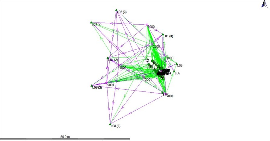
VOS is typically conducted using survey-grade total stations, either in dry docks or on floating dry docks. Fig. 1 illustrates a typical survey network for a 29-foot survey launch secured on a trailer, covering all hydrographic systems. For the purposes of this study, only one sensor was analyzed to ensure efficiency and allow sufficient time for the multiple sets of observations required for the analysis.

In the first experimental setup, the IMU was selected as the sensor for observation. Generally, the IMU has the smallest physical footprint but the most stringent angular accuracy requirements, with a particular focus on roll, which demands an uncertainty of ±0.02°; for example, in the case of the Applanix POS MV WaveMaster with RTK (Applanix, 2015). In the second experimental setup, a circular transducer (Simrad EC150) was chosen, which similarly requires a VOS uncertainty of ±0.02° in both roll and pitch (Simrad, 2019).

The following sections detail the general setup and methodology used for both experiments, focusing on ensuring the required angular accuracy and facilitating reliable comparisons between the sensor setups.

2.1 Experimental setup 1: IMU

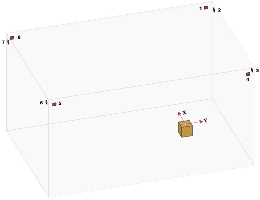
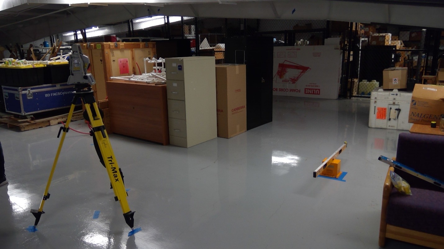
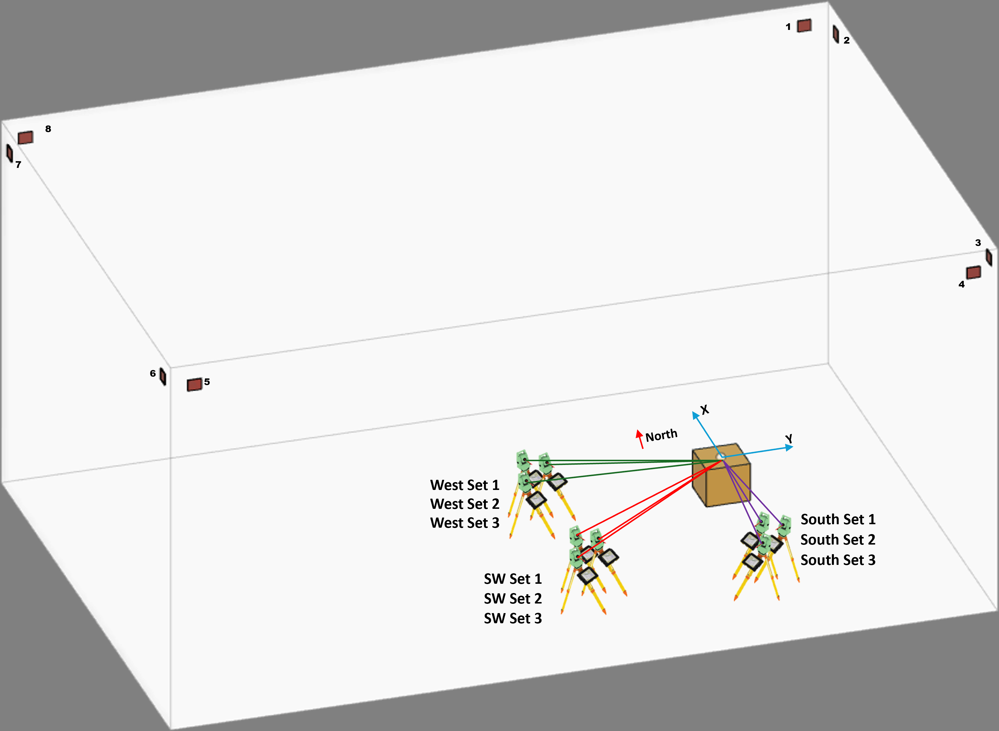
In the first experimental setup, an IMU was placed in a stable, quiet storage room to ensure no movement during the one-week data collection period. Eight reference targets were positioned approximately two meters above the IMU at four corners around it (Sokkia 30 mm reflective tape) (Fig. 2). Fig. 3 shows the photograph of the experimental setup. The setup involved observing all eight reference targets and then collecting measurements from specific points on the IMU, including a level placed flush to the IMU base plate, to calculate roll, pitch, and yaw angles.

A Sokkia Net05AXII industrial total station was used for the experiment. The manufacturer-specified accuracy of the total station is 0.5 mm + 1 ppm for distance measurements and 0.5” for angular measurements (SOKKIA, 2022). The total station was calibrated by a Sokkia certified servicing center eight months prior to this study. The total station measures three basic observables: slope distance, vertical angle, and horizontal angle from the phase center of the instrument to the back of a reflective target. Using trigonometric calculations and applying corrections for environmental factors, these observed quantities were converted by the algorithm inside the total station processor into 3D Cartesian coordinates relative to the origin of the defined local coordinate system.

When doing measurements to compute coordinates of a single point, direct and indirect observations were conducted to minimize residual systematic errors, once with the vertical circle of the total station on the left side of the telescope (known as “face-left” or direct observation) and once with the telescope rotated 180° and the vertical circle on the right (known as “face-right” or indirect observation) (Ghilani & Wolf, 2012). One distance measurement was taken in both face-left and face-right positions, and the average distance was used in the computation. These direct and indirect observations were mathematically adjusted to correct for any residual systematic errors caused by instrument inaccuracies, and the final 3D coordinates of the measured points were calculated. In this context, one observation refers to the combined, adjusted results from both face-left and face-right observations.

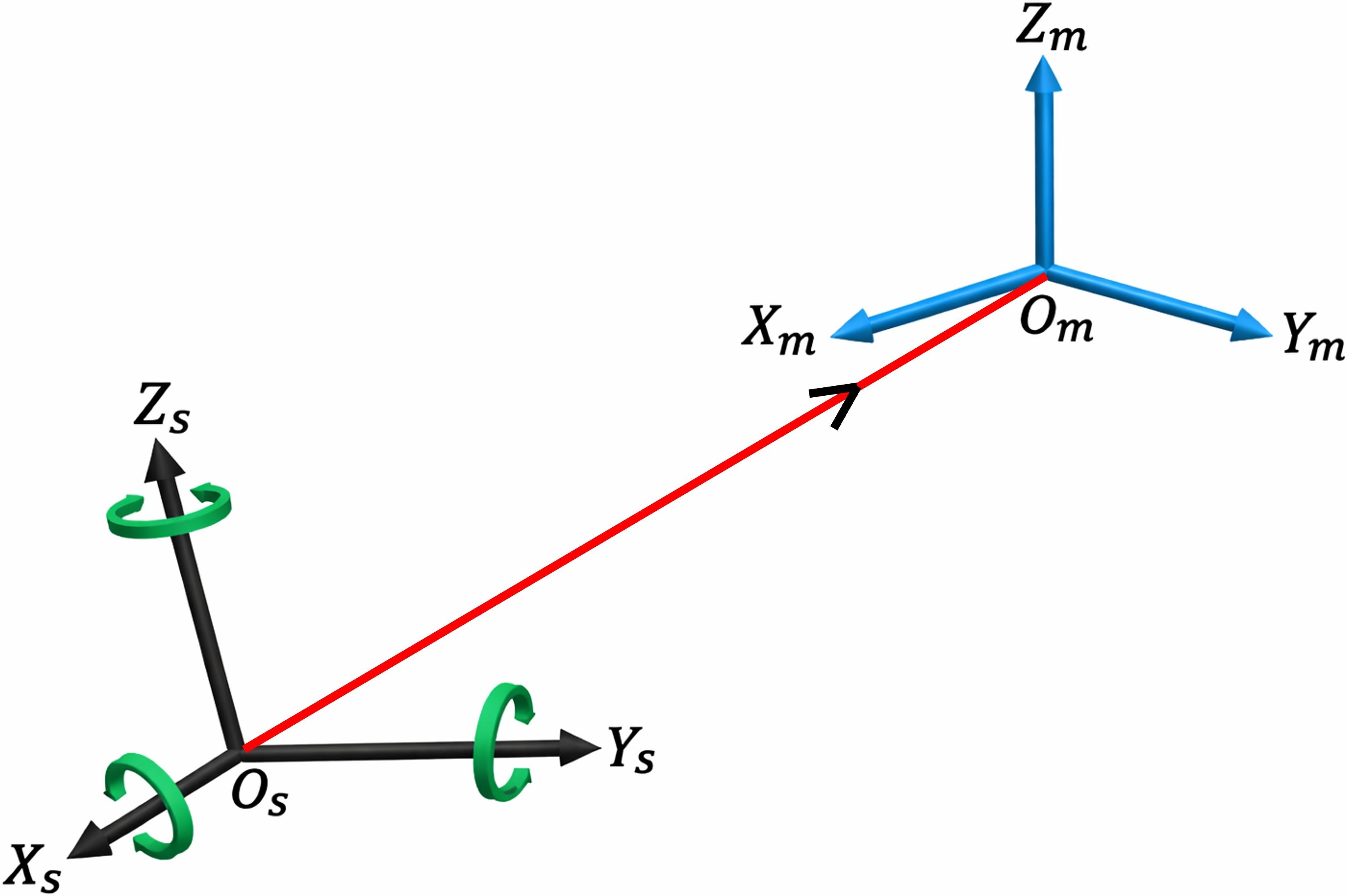
For each total station setup, a unique coordinate system was defined using a fixed offset (100 m North, 100 m East, and 10 m up) from the point of occupation and setting the azimuth to 0° while pointing roughly towards North. This approach avoided using the real-time resection method for station setup and ensured that each setup remained independent, reflecting real-world VOS scenarios where resection or coordinate transformation is typically handled in post-processing. A custom Python script using the singular value decomposition method was developed to compute the six parameters required for coordinate transformation between systems, with flexibility in considering a variable number of common points between the two coordinate systems. The script also performed the coordinate transformation and produced the transformed coordinates of subsequent setups (called slave) in the coordinate system of the first setup (taken as master). As the experiment did not involve any ship, the first setup (master) was treated as the VRF. A schematic of the transformation is provided in Fig. 4.

2.2 Measurements for computing roll, pitch, and yaw angles

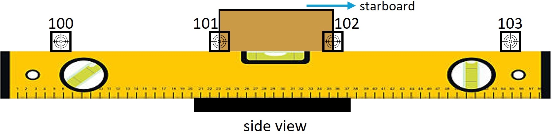
During each setup, coordinates of multiple points were measured on a level to calculate the roll, pitch, and yaw angles of the IMU. A single 20 mm cube with one standard Sokkia 20 mm reflective tape with 0.3 mm target lines on one side was used as the target for these measurements. The cube was placed on top of a 1 m long-level to extend the baseline of the smaller IMU, enhancing measurement precision. No observations of any type using the bubble level were taken for this experiment. The level should preferably be placed on manufacturer-recommended reference surfaces or designated reference points. However, because the reference base plate was not available in this experiment, the level was placed directly on top of the IMU, as shown in Fig. 5.

For roll calculations, the level was positioned approximately aligned along the east (Y) axis on top of the IMU, while for pitch, the level was approximately aligned along the north (X) axis. Any deviation from the exact Y or X axis when making the observations will not impact final computed roll and pitch values, as the measured points are projected onto the YZ plane for roll and onto the XZ plane for pitch. To measure yaw, the level was placed flush with the base of the IMU along either the north (X) axis or with the east (Y) axis, depending on the location of the total station, ensuring a clear line of sight. The IMU manufacturer explicitly identifies these edges as the reference edge for heading alignment measurements. For each orientation, the cube was spaced equally along the length of the level, allowing measurements of four points on the level. Regardless of the total station’s position, the cube was always oriented perpendicular to the line of sight to maintain measurement consistency.

From each station setup, measurements were taken to points needed to compute roll, pitch, and yaw, along with the eight reference marks on the walls. A total of nine different setups were observed, with three setups taken from the South, Southwest, and West directions, as illustrated in Fig. 6. These varied locations ensured comprehensive spatial coverage and allowed for precise calculation of the IMU’s angular offsets.

2.3 Computing roll, pitch, and yaw angles

Once all setups were transformed to the coordinate system of the first setup (master setup), the roll, pitch, and yaw angles between the master coordinate frame and the IMU’s coordinate frame were calculated. A dedicated Python script was developed to handle these computations, providing the flexibility to specify the number of points on the level to be used for angle calculations. When more than two points were used, a 3D least squares line fitting was applied to the measured points. This fitted line was then used to compute the inclination angles (roll, pitch, or yaw) relative to the coordinate system of the master setup, which is taken as the VRF in this context. The measured inclination angles are then converted to the corresponding mounting rotation angles required for system configuration. In practice, this conversion is typically performed using a built-in utility or wizard provided in the IMU manufacturer’s configuration software. The procedure used for this conversion is beyond the scope of the present study.

A set of results obtained from the custom Python script were cross-validated against calculations performed using commercially available software (Coulson, 2024). The differences between the two methods were in the order of 10^−5°, making them negligible and confirming the achievable accuracy using the developed script.

The combination of the nine different setups, the four targets on the level, and the eight reference targets provided multiple variables that could be analyzed for their influence on the computed roll, pitch, and yaw values. This setup enabled a comprehensive examination of how different observational configurations and reference points affected the uncertainty of the angular measurements.

2.4 Experimental setup 2: EC150 transducer face

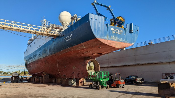
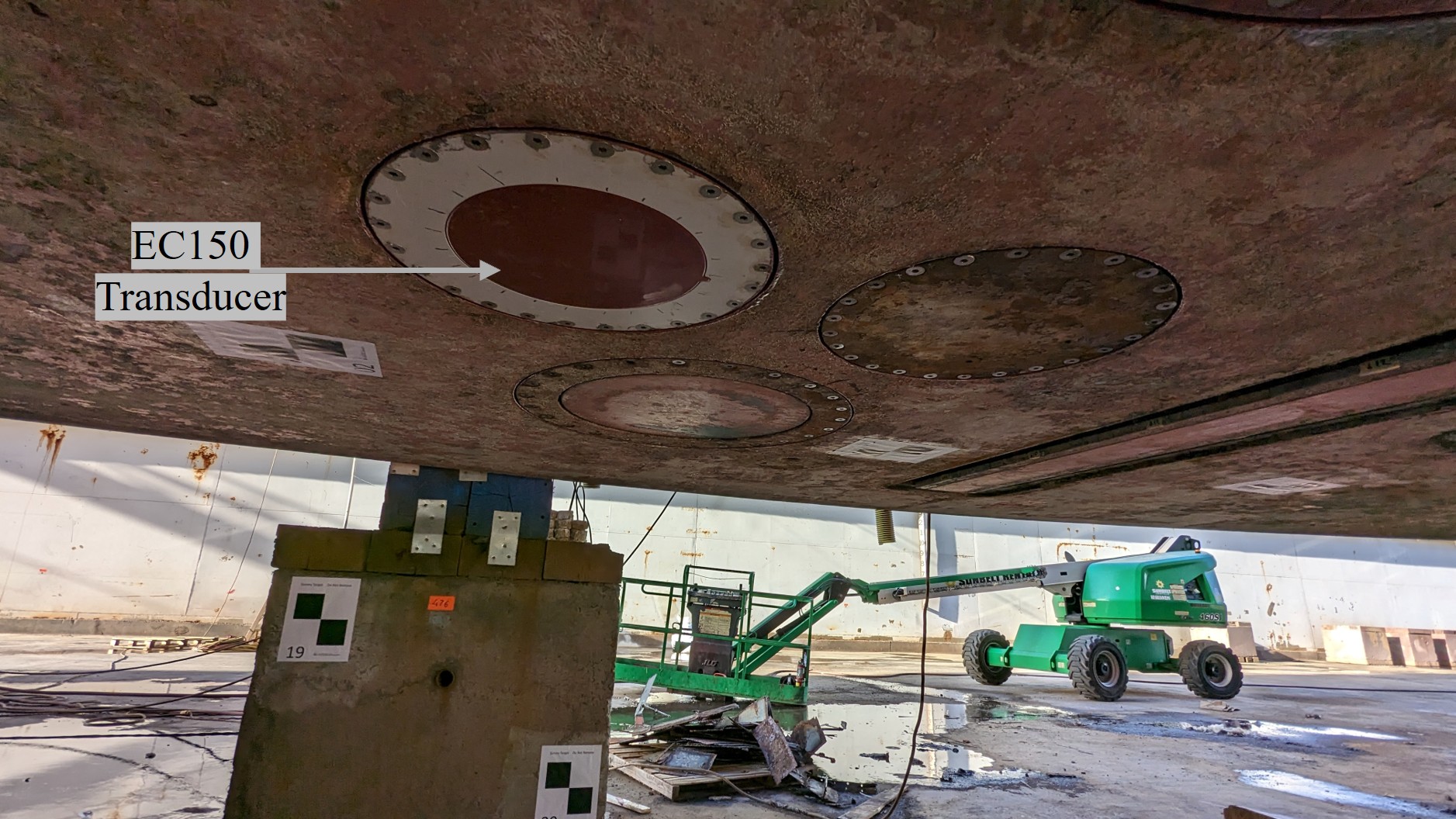
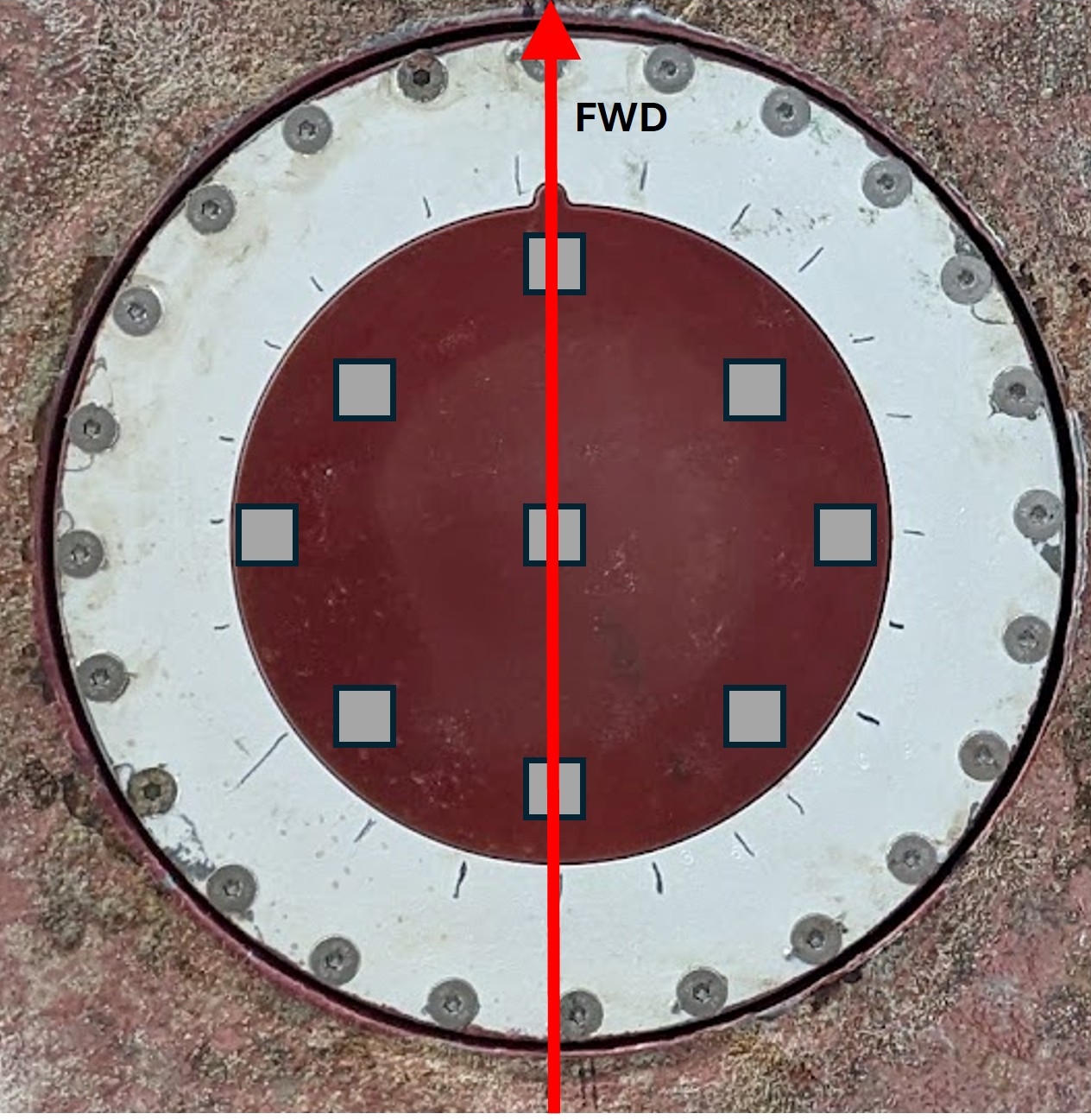
This experimental data collection was part of an actual VOS for the EV Nautilus, which was in a floating dry dock as seen in Fig. 7. The same Sokkia NET05AXII industrial total station used for experimental setup 1 was used for all observations. A new sonar, the Simrad EC150, had been installed at the bottom of the keel (Fig. 8). The primary objective of this VOS was to accurately determine the position and orientation of the EC150 transducer with a diameter of 346 mm (Simrad, 2019) relative to the previously established VRF.

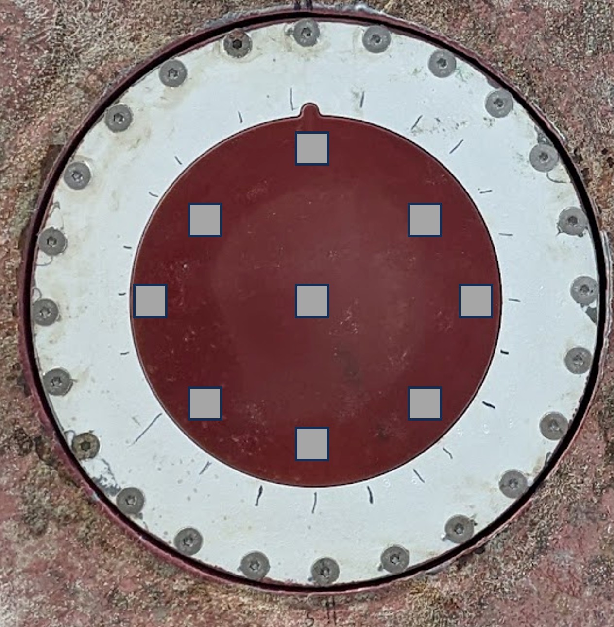
For this purpose, coordinates of nine evenly distributed points on the face of the EC150 transducer (Fig. 9) were collected from three independent total station setups. Three total station setup locations were selected around the EC150: one forward of the EC150 near the vessel centerline, one to starboard of the EC150 across the centerline, and one aft of the EC150 near the vessel centerline. These locations were selected to maximize direct line-of-sight visibility to the EC150 transducer face and a minimum of eight previously established control points. The transducer face was recessed compared to the vessel’s keel, which prevented straightforward extension of the plane of the transducer’s bottom face using a level similar to one done in experimental setup 1 (IMU). This experimental setup was ideal for evaluating the effectiveness of roll and pitch calculations using a fitted plane to the points on the circular transducer face compared to the shorter baseline available.

3 Data analysis, results, and discussion

This section is divided into subsections, and each has a focus on analyzing the impact of different parameters on the uncertainty of the VOS. To maintain clarity and conciseness, only the results for one of the computed angles, either roll or pitch, whichever has the most stringent uncertainty requirements, are discussed below.

3.1 Instrument accuracy

To investigate the effect of instrument accuracy on the VOS results, the ideal approach to obtain real-world values would be to collect parallel datasets using a separate instrument with lower accuracy. However, due to time constraints and the complexity of data collection, a Monte Carlo based simulation approach was adopted instead. Specifically, to simulate results from an instrument with accuracy of ±1” for angular measurement and ±1 mm for linear measurements, the raw measurements from the Sokkia Net05AXII were modified to simulate lower-accuracy results. This was achieved by adding normally distributed random errors of ±0.866” for angular measurements and ±0.866 mm for linear measurements to the raw measurements from the Sokkia Net05AXII with stated manufacturer’s accuracy of ±0.5” for angular measurements and ±0.5 mm + 1 PPM for linear measurements. The expected random error after this simulation is ±1 for angular measurements in seconds and linear measurements in mm. A total of 11 simulated datasets were generated each containing 9 observations, resulting in 99 simulated estimates of the IMU mounting angles.

This approach ensured that all random observational errors present in the original data remained consistent, with the only variable being the simulated random instrument errors. The modified measurements were then used to compute the final 3D point coordinates. These modified datasets, incorporating the added random errors, were subsequently processed in the same manner as the original data to compute the roll, pitch, and yaw of the IMU. The results of this analysis are summarized in Tables 3 and 4.

All consecutive results in this section are arranged in a similar manner to Table 3. The table is organized into two primary sections: Computed angle values and Statistics. Each row corresponds to a specific location, denoted as S (South), SW (Southwest), and W (West), while each column represents either a computed value from a setup or a statistical metric.

The computed angle values section displays the computed roll from three distinct experimental setups labeled Setup1, Setup2, and Setup3. For each location, the table lists three corresponding roll values derived from these setups. These values represent the core data from which the subsequent statistical analysis is drawn. The headers from the statistic sections are self-explanatory and offer a summary of computed values for each location (by row). The last row in green-colored values in the statistic section summarizes the statistics for nine roll values from the three locations and three setups per location. This structured organization allows for an intuitive comparison between the different setups and locations, as well as a clear understanding of the statistical characteristics of the computed values. Please note that all values in the presented tables are expressed in degrees unless specified otherwise.

The average roll angle of -0.27°, as seen in the last row in Table 3, and the average roll value of -0.29°, as seen in the last row in Table 4 indicate that, for the simulated observation scheme used in this study, there is no substantial difference in the estimated mean roll angle when using the higher-accuracy instrument data and the simulated lower accuracy observations. However, a substantial difference is observed in the standard deviation of the individual roll estimates between the two cases (0.05° versus 0.15°).

However, the standard error of the mean obtained from 9 original observations in Table 3 is ±0.017° (0.05 /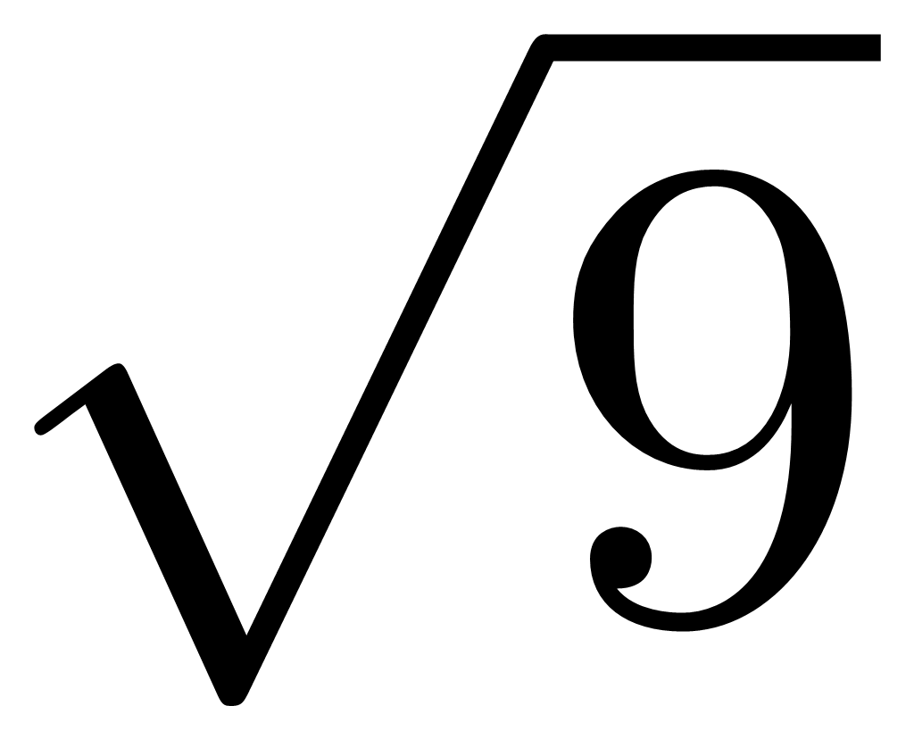), while the corresponding value obtained from 99 simulated observations in Table 4 is ±0.015° (0.15 /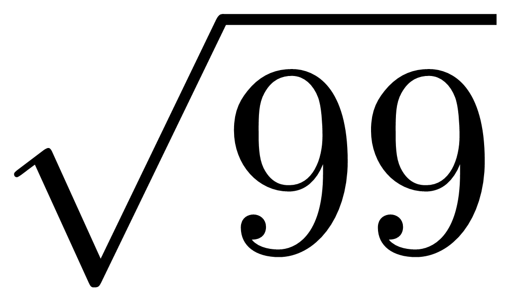) and both values are within the required tolerance of ±0.02°. These standard errors of the mean represent the Type A standard uncertainty of the estimated roll angle referred to hereafter in this paper as the Type A standard uncertainty and were calculated from repeated observations in accordance with the Guide to the Expression of Uncertainty in Measurement (JCGM, 2008). This indicates that a lower-accuracy instrument may still yield a comparable uncertainty in the estimated mean roll angle if a sufficiently large number of observations is acquired. However, in practical field applications, acquiring 99 observations for a single sensor is not realistic, and even the 9 setups used in this experiment may be difficult to achieve under routine survey conditions.

Table 5 presents results obtained by randomly selecting 9 observations from the 99 simulated observations, thereby matching the number of observations acquired with the higher-accuracy total station. Although the estimated mean roll value remains comparable (-0.27°) between the two instrument-accuracy cases, the Type A standard uncertainty increases substantially to 0.053° (0.16 / ) for the simulated lower-accuracy instrument. This indicates that, when the number of observations is held constant, the lower-accuracy instrument does not meet the manufacturer’s 0.02° uncertainty expectation.

The standard error of the mean is ±0.017° in the case of Table 3 and ±0.015° in the case of Table 4. Since all other parameters remained constant between the two sets of observations, the simulated reduction in instrument accuracy did not materially affect the uncertainty of the estimated mean roll value when a sufficiently large number of observations was used. This suggests that, in this case, the effect of increased observational redundancy compensated for the lower nominal instrument accuracy. Consequently, the simulated lower-accuracy instrument, with approximately 1” angular and 1 mm linear accuracy, produced a comparable Type A standard uncertainty in the estimated mean roll angle to that obtained from the higher-accuracy Sokkia NET05AXII. However, this comparison is based on 9 observations obtained with the higher-accuracy instrument and 99 simulated observations representing the lower-accuracy instrument. In practical field applications, acquiring such a large number of observations for a single sensor installation is generally not feasible. Therefore, instrument selection should be based not only on the required uncertainty of the final result but also on the practical number of observations that can realistically be acquired in the field.

3.2 Direct and indirect observations

The next parameter examined during the experiment was the effect of using direct-only observations versus both direct and indirect observations. As previously discussed, combining adjusted direct and indirect observations helps to eliminate any residual internal instrument systematic errors (Schofield, 2001) after calibration, while also minimizing the impact of random errors, such as pointing errors. In the field, both direct and indirect observations were performed for each angle and distance measurement targeting a single cube on a level. The resulting computed roll values are presented in Table 3. To assess the 3D position values based solely on direct observations, the indirect observations were manually removed from the raw data prior to calculating the 3D positions of the points. These points were then used to compute the roll values based on direct observations alone, as shown in Table 6.

As shown in the last row of Tables 3 and 6 (green-colored), the mean roll angle differs by only 0.01° between the two results (-0.27° and -0.28°). The standard deviation computed from the nine observations remains consistent at 0.05° in both cases. This suggests that, at relatively short distances (approximately 3 meters in this case), the residual systematic errors in horizontal and vertical angles, stemming from instrument inaccuracies such as collimation error, misalignment in the horizontal plane of rotation, or the vertical plane not being exactly perpendicular, with the used total station (with its magnitude of calibration parameters) and in this particular scenario, do not significantly impact the results. However, this finding may change in the presence of larger systematic errors or when observations are made over longer distances. Additionally, this implies that when instruments are calibrated by a certified servicing center and subsequently verified on-site by the surveyor prior to data acquisition, surveyors can rely on direct observations alone for shorter distances. Nevertheless, prior to data acquisition, the calibration parameters should be verified by the surveyor to ensure the integrity and reliability of the measurements, particularly in applications demanding high accuracy. When operational time permits, performing direct and indirect observations is advisable, as this practice further enhances measurement precision and robustness.

3.3 Baseline length

The accuracy of 3D point coordinates on the level is largely independent of the distance between the points. However, the angular offset is computed from the relative positions of the points. Therefore, for the same angular offset, a longer distance between the points (i.e., a longer baseline) should, in theory, reduce the influence of coordinate uncertainty and improve the accuracy of the estimated offset. The authors have observed that, while it is possible to extend baseline lengths using a precise level or any other machined flat surface, surveyors do not always take advantage of this option. In most cases, the shortest baselines are observed with IMUs, where the reference base plate is relatively short (10–30 cm). However, using a precise flat surface, the baseline can be extended to 1 meter or more, provided there are no obstructions such as bulkhead walls or mounting screws.

To quantify any improvement in precision with a larger baseline, selective points were used to compute the angular offsets. As previously described, four equally spaced points were measured on the level from each setup (see Fig. 5). This allowed the innermost two points (101 and 102) to be used for the computation of roll offsets (see Table 3) with a shorter baseline, while the outermost two points (100 and 103) were used to compute a second set of roll offsets (Table 7) with a longer baseline. The difference between these two sets of angular offsets was used to assess the improvement in standard deviation.

Upon reviewing Tables 3 (short baseline) and 7 (long baseline), it is evident that the final mean roll value (shown green-colored in the last row of the tables) for the short baseline is -0.27° with a standard deviation of 0.05°, while for the longer baseline it is -0.23° with a standard deviation of 0.04°. Although the improvement in standard deviation is small, the mean value changes by 0.04°, which is notable relative to the required roll uncertainty of ±0.02°. The difference between the minimum and maximum values for the short baseline is 0.19°, compared to 0.11° for the long baseline. If only one observation were performed, the min-max difference obtained from the set of nine observations represents the possible range of the resulting roll value. This range is smaller for the longer baseline, indicating lower variability in the estimated roll values compared with the shorter baseline for the observations considered in this study.

Although the standard deviation of the individual observations (0.04° for the long baseline and 0.05° for the short baseline) exceeds the required roll tolerance of ±0.02° for both configurations, the Type A standard uncertainty obtained from nine observations is ±0.013° for the longer baseline and ±0.017° for the shorter baseline. These values are within the required tolerance. The longer baseline, therefore, provides a smaller uncertainty. Furthermore, the standard deviation of the mean can be reduced either by increasing the number of observations or by eliminating outlier roll values, as discussed in Section 3.7.

3.4 Number of points on the baseline

This section analyzes any improvements in the final mean roll value resulting from measuring multiple points along a baseline. As previously described, a total of four points were measured on the level during data collection. One set of roll values was computed using the two outermost points (Table 7), while another set of roll values

Table 8 was calculated using a best-fitting 3D line through all four points. The mean roll values from Table 7 (-0.23°) and Table 8 (-0.24°) are nearly identical, both with a standard deviation of 0.04°. Using only two points, particularly the outermost points, introduces higher sensitivity to outliers, as these points act as leverage points and strongly influence the fitted line. Therefore, including additional points provides redundancy and allows potential outliers to be detected during post-processing. However, in this case, the nearly identical mean roll values suggest that no outliers are present. Under this assumption, the results indicate that the number of points used in the roll computation has an insignificant effect on the uncertainty of the computed roll. Instead, the baseline length plays a more significant role in determining the uncertainty than the number of points measured on the baseline, as discussed in Section 3.3.

3.5 Number of reference points

In geodetic network adjustment, the precision of estimated parameters, in this case the roll value, is influenced by both the number of observations and the spatial distribution (geometry) of the reference points. A limited point distribution can weaken the network geometry and increase the uncertainty of the transformation parameters and ultimately that of the roll value. As previously described, nine independent local setups were established in their respective coordinate systems. One setup was selected as the master coordinate system, and the remaining eight setups were transformed into this system using observations to eight common reference points. This section investigates the impact of the number of reference points used during the transformation on the computed mean roll values. For the roll values presented in Table 9, only three reference points (6, 7, and 8) were used during the transformation. Although this configuration results in a limited spatial distribution of reference points, it was intentionally selected to represent constrained measurement geometries that may occur in practical environments, such as narrow corridors or hallways, where observations are often performed. This configuration, therefore, represents a near worst-case scenario. The positions of the two outermost targets on the level were then used to compute the associated roll value. A similar process was applied using all eight reference points, resulting in the roll values shown in Table 7.

As shown in Table 9, using three reference points yielded a mean roll value of -0.25°, with a standard deviation of the observations of 0.05° (last row of the table in green color). According to Table 7, when all eight reference points were used, the mean roll value is -0.23°, while the standard deviation of the observations decreased slightly to 0.04°. The corresponding standard deviation of the mean is approximately 0.017° for the three-reference point configuration and 0.013° when eight reference points are used. These results indicate that, in this case, using eight reference points yields only a small reduction in uncertainty compared with using the three reference points in Table 9. This suggests that the positional errors of the three reference points are small and that the number of reference points has a limited influence on the computed roll values. Similar behavior was observed for the pitch and yaw values.

However, this may not always be the case in field conditions. If one of the three reference points had a relatively large positional error, it would likely impact the accuracy of the computed roll values. Using multiple reference points minimizes the influence of error from any single reference point through least squares estimation, and any erroneous reference point can be identified by higher residual values following the least squares adjustment. Another important consideration when using three reference points is their orientation. The orientation of the reference points relative to the total station can affect how positional errors associated with the reference points affect the positional error of the total station computed using the resection process. Furthermore, the orientation of the IMU with respect to the total station will influence how positional errors in the total station translate to the position of the targets on the level.

In practical field conditions, surveyors are often constrained by restricted geometry, leading to orientations similar to those used in this case. Therefore, it is essential to use multiple reference points to account for both the orientation of the total station with respect to the reference points and to identify and eliminate any high-error reference points during the computation process.

3.6 Effect of the location of the total station

This section examines the influence of the observation location on the computed orientation parameters. Roll, pitch, and yaw values were computed for three different measurement locations (S, SW, and W), each based on three independent setups. The resulting values and their associated statistics are presented to evaluate the variability of the estimated parameters for the different observation configurations.

Upon reviewing the tables presented in the analysis (from Tables 3 to 9), it is evident that the S and W orientations consistently exhibit lower standard deviations (shown in the last column, not green-colored) compared to the SW orientation, indicating that, for roll-angle estimation, the S and W station locations yielded lower variability than the SW location. However, no such pattern was observed in the case of pitch (Table 10) and yaw (Table 11) computations.

Table 10 presents the computed pitch values and associated statistics for the three measurement locations (S, SW, and W). The S and SW locations exhibit comparable variability, each yielding a standard deviation of 0.03° across the three setups, whereas the W location shows a smaller standard deviation of 0.01°. This behavior differs from that observed for the roll values, where the S and W locations generally exhibited lower variability than the SW orientation.

Table 11 presents the computed yaw values and associated statistics for the three measurement locations (S, SW, and W). The S location exhibits the largest variability, with a standard deviation of 0.06°, while the SW and W locations show smaller standard deviations of 0.03° and 0.02°, respectively. This behavior also differs from that observed for the roll values, where the S and W locations generally exhibited lower variability than the SW orientation.

Given the limited number of observations per location, these results should be interpreted cautiously. With the available data, it is not possible to conclusively determine whether the station location relative to the sensor has a measurable influence on the computed orientation angles. Further field testing, involving a greater number of setups and longer distances, is necessary to draw definitive conclusions.

3.7 Number of station setups: variability and outlier assessment

For this analysis, the means and standard deviations from Table 7 are used. When analyzing the Setup1 values for the three orientations (S, SW, and W), the obtained roll values are -0.27°, -0.32°, and -0.22°. These observations yield a mean roll value of -0.27° with a standard deviation of the observations of approximately 0.05°. The corresponding standard deviation of the mean, representing the Type A standard uncertainty, is approximately 0.03°. This value exceeds the required uncertainty threshold of 0.02°, indicating that additional independent observations from further station setups would be required to achieve the desired uncertainty level. Additionally, no potential outliers can be identified among the three roll values (-0.27°, -0.32°, and -0.22°), as all observations lie within one standard deviation of the mean value (-0.27°); therefore, none of the observations can be reasonably excluded from the analysis.

When analyzing the Setup2 values for the three orientations (S, SW, and W), the roll observations (-0.22°, -0.21°, and -0.21°) yield a standard deviation of approximately 0.01°. The corresponding standard deviation of the mean is approximately 0.003°, which is below the required uncertainty threshold of 0.02°. A similar result is obtained for Setup3, where the observations (-0.22°, -0.22°, and -0.23°) yield a standard deviation of approximately 0.01° and a standard deviation of the mean of approximately 0.003°.

When three independent angle values, either from different orientations or from different setups, do not meet the required minimum uncertainty threshold, the observations can be examined for potential outliers by evaluating their deviation from the mean relative to the standard deviation of the observations. A new mean and standard deviation can then be calculated using the remaining two values and compared against the required minimum standard deviation. This situation occurs when considering the three setups for the SW orientation, where the value of -0.32° shows the largest deviation from the mean and can be treated as a potential outlier. After excluding this value, the recalculated mean becomes -0.21° with a standard deviation of approximately 0.01°.

Similarly, for the three setups from the S orientation, the value of -0.27° can be considered an outlier, resulting in a standard deviation of 0.00° when excluded.

3.8 Using a fitted plane to compute roll and pitch

To quantify precision and Type A uncertainty in the obtained angles using plane fitting compared to line fitting, data collected for the VOS of EV Nautilus was analyzed. Table 12 presents the pitch values derived using three different methods. Please note that for the EC150 transducer, the required accuracy for roll and pitch mounting angle estimation is 0.02°. For all three methods, the coordinates of the points are initially measured in local coordinate frames and subsequently transformed into the vessel’s coordinate frame before computing the pitch and roll angle values.

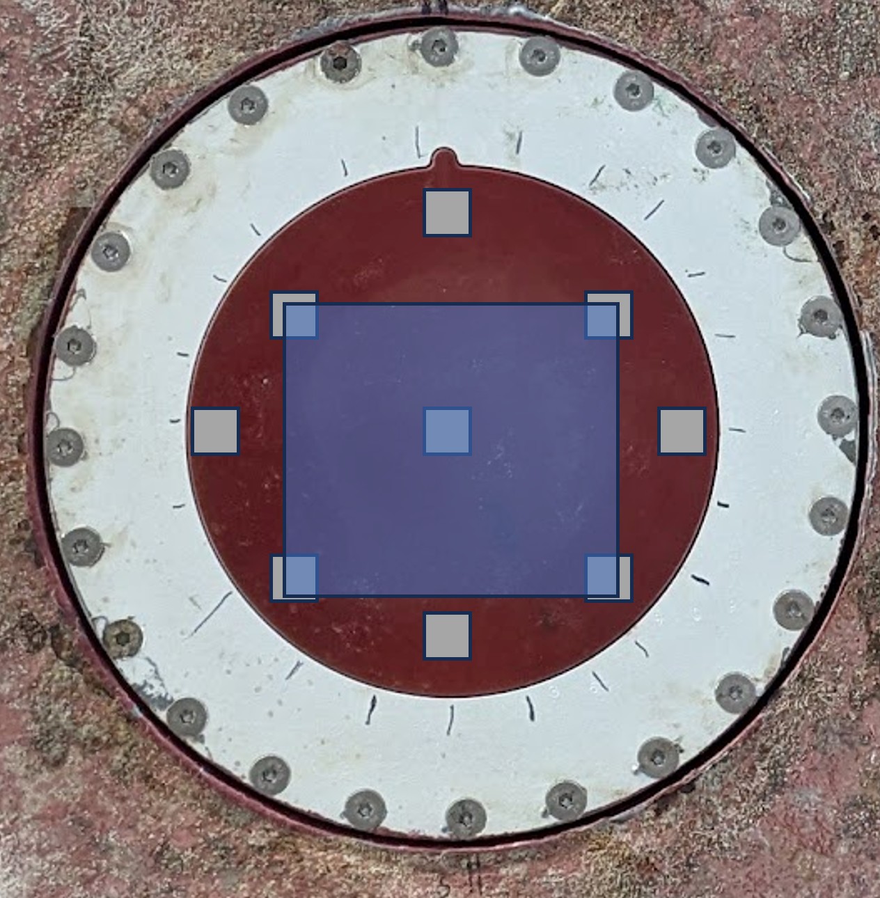
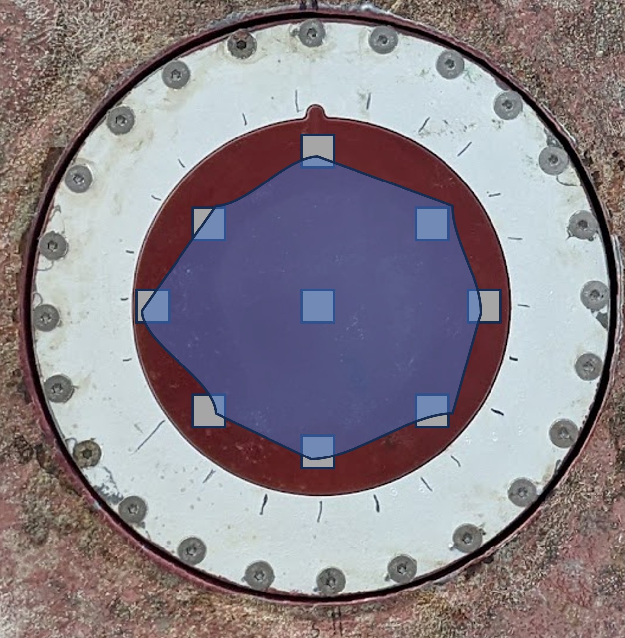
The first method utilizes a 3D line best fitted to the along-track points on the face of the EC150 transducer (as shown in Fig. 10a). The fitted line represents the longitudinal orientation of the transducer. To compute the pitch angle, the fitted line is projected onto the vessel’s XZ plane (forward–down), eliminating the Y (across-track) component. The pitch angle is then derived from the slope of this projected line relative to the vessel’s longitudinal (X) axis. The second method involves a normal vector to a 3D best-fit plane, fitted using four out of nine points measured on the face of the transducer (Fig. 10b). The third method uses a normal vector to a 3D best-fit plane fitted to all nine points on the transducer’s surface (Fig. 10c). In the second and third methods, the normal vector is projected onto the vessel’s XZ plane (forward–down), and the pitch angle is computed as the angle between the projected normal vector and the Z axis of the vessel reference frame. The orientation angles are derived from geometric relationships between the measured point coordinates and the vessel reference frame. The direction vector of the fitted line or the normal vector of the fitted plane defines the orientation of the transducer surface, from which the pitch and roll angles are computed.

From Table 12, it can be observed that the standard deviation is highest for the first method, which uses only three points in the along-track direction. The standard deviation decreases to 0.03° for the second method, which fits a plane using four points, and further decreases to 0.01° for the third method, which fits a plane using all nine points to compute the pitch angle. The corresponding standard deviation of the mean (Type A standard uncertainty for three samples) is approximately 0.029°, 0.017°, and 0.006° for the three methods, respectively. Similar improvements were observed for the roll angle.

It should be noted that the face of the EC150 transducer is designed to be planar; therefore, fitting a plane to multiple points on the transducer surface provides a stable estimate of its orientation. These results indicate that for circular transducers, such as the EC150, using the normal vector of a fitted plane to multiple points on the transducer surface provides improved roll and pitch estimations. This approach is particularly advantageous when physical constraints restrict the use of a level to extend the baseline length of the transducer for improving the accuracy of angle measurements.

4 Conclusions

Although a priori and a posteriori uncertainty analysis can be derived from the mathematical relationships between measured quantities and estimated parameters, this study focused on quantifying the variation of the final estimated installation parameters through simulated and real-world observations. Two complementary case studies were used. A simulated IMU configuration was employed to evaluate the influence of survey design and measurement factors on the precision of the estimated parameters, while field measurements from EV Nautilus were used to assess the influence of the computation method on the precision of roll and pitch estimates. Collectively, these analyses provide insight into how observation strategy, measurement geometry, redundancy, and processing methodology influence the precision and Type A standard uncertainty of the estimated orientation parameters obtained during VOS.

4.1 Observation method and instrument factors (instrument accuracy and direct–indirect observations)

Within the short-distance experimental configuration tested in this study, instrument accuracy had a measurable influence on the precision of the estimated parameters, whereas the use of direct versus combined direct–indirect observations did not produce a measurable change in the estimated angles or in their associated precision metrics, including the standard deviation of the observations and the Type A standard uncertainty. Under the tested conditions, observations obtained with the higher-accuracy instrument (0.5”/0.5 mm) using 9 observations and simulated lower-accuracy observations (1”/1 mm) using 99 observations produced comparable mean angular estimates and comparable Type A standard uncertainties. However, when the number of observations was held constant, the higher-accuracy instrument provided lower Type A uncertainty and therefore greater confidence in the estimated parameters than a randomly selected subset of 9 observations from the simulated lower-accuracy datasets. This indicates that lower nominal instrument accuracy may be compensated for by substantially increasing the number of observations, although such observation counts are often impractical in field applications.

By contrast, the use of only direct observations did not produce a significant increase in the uncertainty of the estimated parameters under the conditions of this experiment setup, suggesting that random observational variability had a greater influence on the final estimates than the residual systematic errors remaining after instrument calibration. This observation is limited to the tested configuration and does not reduce the importance of identifying and minimizing systematic errors in general survey practice. Systematic effects, typically mitigated through direct–indirect observations, were likely small in this case because of the short observation distances and the limited range of zenith angles. In practical vessel installations, however, different sensors may be observed under different geometric configurations and zenith-angle ranges, which may increase sensitivity to systematic deviations. Accordingly, standard survey practice should still include the use of instruments with appropriate nominal accuracy, proper factory and field calibration, and direct–indirect observations.

4.2 Baseline geometry (baseline length and number of points on baseline)

Baseline length had an influence on the precision of the estimated roll offsets. As expected, longer baselines reduced the standard deviation of the estimated parameters because the same linear measurement uncertainty translated into a smaller angular uncertainty. In contrast, increasing the number of points used to define the baseline from two to four did not produce a noticeable reduction in the dispersion of the estimated roll values under the tested conditions. These results are specific to the baseline lengths and geometry evaluated in this study. In practical survey applications, extending the baseline length is beneficial when feasible, whereas the number of points used to define the baseline should be selected based on redundancy needs, site constraints, and the expected gain in precision.

4.3 Reference geometry and instrument location (number of reference points and location of the total station)

Within the tested short-range configuration, increasing the number of reference points from three to eight did not significantly improve the precision of the estimated parameters, and the location of the total station relative to the measured object did not produce a measurable change in the estimated angles. These outcomes are specific to the experimental measurement configuration evaluated in this study. In theory, a larger number of reference points strengthens the observation network and reduces sensitivity to individual point-coordinate errors; however, in this case, the positional errors of the three reference points were small, which likely limited any observable improvement in the computed roll values. The available data also does not permit a conclusive assessment of the influence of station location, as the number of observations per station location was limited. Nevertheless, using only the minimum of three reference points is not recommended in practice because it provides no redundancy for identifying point-coordinate errors during post-processing. Additional, well-distributed reference points enable least-squares adjustment and improved detection of positional inconsistencies when transforming local coordinates into the master coordinate system. This analysis was performed for a single sensor and therefore does not evaluate the full internal vessel sensor network.

4.4 Observation redundancy and quality control

Observation redundancy (number of station setups) had a direct influence on the precision of the estimated roll value and on the ability to identify potential outliers. Nine independent station setups were analyzed to examine how the standard deviation of the derived roll values changed with the number of setups. In the tested configuration, two independent setups with different orientations were sufficient to produce roll estimates with a standard deviation below 0.02°. However, this standard deviation reflects only the precision of the estimated roll values and not their absolute accuracy. Although two setups were sufficient in this experimental case, reliance on only two observations is not recommended in practical survey work. If one observation is later identified as an outlier during processing, it may not be possible to return to the field and acquire an additional setup. For this reason, at least three independent station setups are recommended in practice to provide redundancy for outlier detection and to improve confidence in the estimated orientation parameters.

4.5 Computation method (fitted plane vs. line fitting)

The computation method had a substantial effect on the precision of the estimated roll and pitch parameters. For sensors or surfaces that can reasonably be treated as planar, fitting a plane to the maximum possible number of observed points produced lower standard deviations and lower Type A standard uncertainties than line fitting or plane fitting with fewer points. This is expected because the fitted-plane approach uses more observations and better represents the full sensor surface geometry, thereby reducing sensitivity to individual point-measurement noise. In contrast, line fitting relies on fewer points and is therefore more sensitive to local observation errors. This effect was especially important for short baselines and for sensors with narrow dimensions in the direction relevant to the angle being estimated.

For non-circular or linear-array sensors, such as multibeam transducers and some IMUs, plane fitting should be used to compute roll and pitch whenever sufficient points are available. When plane fitting is not feasible, such as in constrained spaces around an IMU, a line fit should be used with the longest possible baseline, since increasing baseline length improves the precision of the estimated angles. This is particularly important for roll estimation in narrow multibeam transmitters and pitch estimation in narrow multibeam receiver arrays. For circular sensors such as the EC150, the fitted-plane method based on nine points substantially reduced the Type A standard uncertainty relative to short-baseline line fitting.

For azimuth or heading offset estimation, plane fitting is generally not applicable, and the surveyor must instead use manufacturer-identified edges, marks, or machined reference surfaces, as is often the case for IMU base plates. In such cases, a line fit using the longest feasible baseline should be applied. For circular arrays, including IMUs with circular base plates and circular transducers, baseline extension is often not possible for heading estimation. In these situations, multiple two-point line-based heading measurements should be acquired, and the mean value together with the standard deviation of the observations should be used to estimate the most reliable heading offset and to identify potential outliers. For larger linear transducers, such as lower-frequency sonar arrays, the full length of the transmitter or receiver edge should be used wherever possible to compute along-axis or across-axis heading angular offsets. In practical applications, the choice between plane fitting and line fitting should therefore be guided by actual sensor geometry, available access, and the number and distribution of observable points.

4.6 Overall implications

Taken together, the results indicate that for short-range VOS configurations, the precision and Type A standard uncertainty of the estimated installation parameters are governed primarily by instrument accuracy, observation geometry, redundancy, and computation method. Within the tested range, lower nominal instrument accuracy can be partially compensated for by increasing the number of observations, but this is often impractical in field conditions. By contrast, the tested direct-only observation strategy did not significantly degrade the estimated uncertainties in this short-range, well-calibrated configuration. Accordingly, instrument selection should be based not only on nominal specifications but also on the number of repeat observations that can realistically be collected, the target uncertainty of the estimated installation parameters, and the expected sensitivity of the observation geometry to residual systematic effects.

These findings do not establish a universal accuracy standard for all hydrographic survey categories under IHO S-44. Rather, they represent a step toward a more standardized and technically defensible methodology for dimensional control vessel offset surveys that can meet or exceed manufacturer requirements and support uncertainty estimates that are traceable and practically achievable. More realistic uncertainty estimates for installation parameters are expected to improve subsequent uncertainty propagation into final bathymetric products, although that propagation was not explicitly evaluated in this study.

4.7 Future work

Future work should examine longer observation distances, broader station geometries, additional sensor configurations, and the propagation of installation-parameter uncertainty into final bathymetric uncertainty in both the vertical and horizontal components. A more rigorous least-squares analysis, including cofactor propagation, redundancy measures, and controllability of observations, would also provide additional insight into the strength of the measurement configuration and the sensitivity of the estimated parameters to observation geometry.

References

Applanix (2015). POS MV WaveMaster II Specifications. Applanix Corporation, Richmond Hill, ON, Canada. https://www.uniquegroup.com/wp-content/uploads/2022/10/POSMV-Spec-Sheet-2015.pdf (last accessed 26 April 2026).

Applanix (2017). POS MV V5 Installation and Operation Guide. Applanix Corporation, Richmond Hill, ON, Canada. https://www.applanix.com (accessed on 1 May 2021).

Applanix (2025). Trimble Applanix POS MV. Applanix Corporation, Richmond Hill, ON, Canada. https://www.applanix.com/products/posmv.htm (last accessed 26 April 2026).

Class of 2023 (2023). Field report for Lemoyne VOS. Hydrographic Science Program, University of Southern Mississippi.

Coulson, A. (2024). SC4W (Survey Calculations 4 Windows). Smith & Coulson Ltd., United Kingdom. https://www.sc4w.com/ (last accessed 26 April 2026).

ELAC Sonar (2021). SB 3050 2G Medium-Depth Multibeam System – For Mapping the Continental Slope. ELAC SONAR GmbH, Kiel, Germany. https://www.elac-sonar.de/fileadmin/content/downloads/sb-3050-2g-product-brochure.pdf (last accessed 26 April 2026).

Ghilani, C. D. and Wolf, P. R. (2012). Elementary surveying: An introduction to geomatics (13^th ed.). Prentice Hall.

Hiroji, A. and Oderinde, O. (2022, December). EV Nautilus vessel offset measurement survey report. School of Ocean Science and Engineering, University of Southern Mississippi, USA.

Hughes Clarke, J. E. (2003). A reassessment of vessel coordinate systems: What is it that we are really aligning? Proceedings of the US Hydrographic Conference, 1–12.

Hughes Clarke, J. E. (2018). Multibeam echosounders. In A. Micallef, S. Krastel and A. Savini (Eds.), Submarine geomorphology (pp. 25–41). Springer International Publishing. https://doi.org/10.1007/978-3-319-57852-1_3

IMTEC Group. (2021, June). RV Sally Ride AGOR-28 EM124 TX/RX, EM712 TX/RX, SBP, ADCP orthogonal coordinate survey.

IHO (2022). Standards for Hydrographic Surveys (Ed. 6.1.0). IHO Special Publication S-44, International Hydrographic Organization, Monaco. https://iho.int/uploads/user/pubs/standards/s-44/S-44_Edition_6.1.0.pdf (last accessed 26 April 2026).

JCGM (2008). Evaluation of measurement data—Guide to the expression of uncertainty in measurement (JCGM 100:2008). Joint Committee for Guides in Metrology. www.bipm.org/documents/20126/2071204/JCGM_100_2008_E.pdf (last accessed 26 April 2026).

Kongsberg (2021, May). Kongsberg EM 304 Installation Manual. Kongsberg Maritime AS, Kongsberg, Norway.

Kongsberg (2024). Kongsberg Seapath 380. Kongsberg Maritime AS, Kongsberg, Norway. https://www.kongsberg.com/discovery/discontinued/seapath-380—utilising-gps-glonass-galileo-beidou-and-qzss/ (last accessed 26 April 2026).

LEICA (2014). Leica FlexLine TS07 Manual Total Station. Leica Geosystems AG, Heerbrugg, Switzerland. https://leica-geosystems.com/-/media/files/leicageosystems/products/datasheets/leica%20flexline%20ts07%200221%20en-in%20lr.pdf (last accessed 26 April 2026).

LEICA (2020). Leica Nova MS60 Data Sheet. Leica Geosystems AG, Heerbrugg, Switzerland. https://leica-geosystems.com/-/media/files/leicageosystems/products/datasheets/leica_nova_ms60_ds.ashx%3Fsc_lang%3Den%26hash%3D74DB2830F27BF20A75AC01710764345D (last accessed 26 April 2026).

MAC (2024). Tech Reports. Multibeam Advisory Committee. https://mac.unols.org/reports/ (last accessed 26 April 2026).

SBG (2025). Discover Apogee Series. SBG Systems, Carrières-sur-Seine, France. https://www.sbg-systems.com/products/apogee-series-high-accuracy-ins-gnss/ (last accessed 26 April 2026).

Schofield, W. (2001). Engineering surveying: Theory and examination problems for students (5^th ed.) Elsevier.

Simrad (2019). Simrad EC150-3C Installation Manual. Kongsberg Maritime AS, Kongsberg, Norway. https://www.simrad.online/td_150/ec150_3c/ec150_3c_ins_en_a4.pdf_ (last accessed 26 April 2026).

SOKKIA (2022). NET05 AXII Industrial Monitoring and Measurement. Sokkia Corporation, Olathe, USA. https://us.sokkia.com/products/optical-instruments/monitoring-specialty-systems/net-ax-industrial-monitoring-and (last accessed 26 April 2026).

Teledyne Marine (2022). HydroSweep Deep-Sea Multibeam Echosounder. Teledyne RESON A/S, Slangerup, Denmark. https://www.teledynemarine.com/en-us/products/SiteAssets/RESON/Hydrosweep%20DS%20product%20leaflet.pdf (last accessed 26 April 2026).

TOPCON (2016). MS AXII Series High Accuracy Measuring Station. Topcon Corporation, Tokyo, Japan. https://www.topconpositioning.com/content/dam/topcon_digital_asset_hub/collateral/brochures/MSSeries_MSAXII_Broch_T547EN_TEAM_EN_EU_HiRes.pdf (last accessed 26 April 2026).

TOPCON (2018, March). Topcon GM-50 Total Station. Topcon Corporation, Tokyo, Japan. https://mytopcon.topconpositioning.com/na/total-stations/manual-total-stations/gm-50 (last accessed 26 April 2026).

TOPCON (2019). NET05AXII, NET1AXII 3D Station. Topcon Corporation, Tokyo, Japan. https://geo-tronics.com/wp-content/uploads/2021/04/Datasheet-NETAXII-1.pdf (last accessed 26 April 2026).

TOPCON (2025). Topcon GT 1201 | Robotic Total Station. Topcon Corporation, Tokyo, Japan. https://www.skippertech.com/product/gt-1201/ (last accessed 26 April 2026).

Trimble (2015). Trimble S9. Trimble Inc., Westminster, USA. https://geospatial.trimble.com/products/hardware/trimble-s9 (last accessed 26 April 2026).

Trimble. (2023). Trimble SX12. Trimble Inc., Westminster, USA. https://geospatial.trimble.com/en/products/hardware/trimble-sx12 (last accessed 26 April 2026).

Vaníček, P. and Krakiwsky, E. J. (2015). Geodesy: The Concepts (2^nd ed.). Elsevier.

Westlake Consultant (2021). RV Okeanos Explorer R337 Survey of Ships Mission and Scientific Equipment.

Authors’ biographies

Anand Hiroji is an Associate Professor of Hydrography in the Division of Marine Science, School of Ocean Science and Engineering, at The University of Southern Mississippi, USA. His research interests include multibeam sonar backscatter optimization and calibration, bathymetric positioning accuracy, uncrewed surface vessels, and hydrographic vessel configuration surveys. He earned a B.E. in Civil Engineering from Shivaji University, India, in 2005, and an M.E. in Geomatics Engineering in 2011 and a Ph.D. in Ocean Mapping in 2016 from the University of New Brunswick, Canada.

Olaoluwa Oderinde is a Category-A Hydrographer with over nine years of experience in offshore hydrographic and marine geophysical surveys. He holds a B.Sc. in Surveying and Geoinformatics from the University of Lagos, Nigeria, and an M.Sc. in Hydrographic Science from the University of Southern Mississippi, USA. His work focuses on high-resolution seabed mapping, geophysical data processing, geohazard identification, and the application of uncrewed survey systems, supporting offshore energy, maritime safety, and coastal resilience initiatives.