1 Introduction

Sidescan sonar is a widely used technology to create high resolution images of the seafloor. It has become an important tool in numerous marine applications, including underwater construction and archaeology, environmental monitoring and offshore energy exploration (Blondel, 2009). Sidescan sonars are also employed by non-profit organisations to help identify human traces, such like the search for litter, anquoring marks etc. (e.g. Díaz-Mendoza et al., 2024; Bruns et al., 2020). The process of converting raw sonar data into informative and interpretable images is necessary in order to make the data usable and requires a full processing chain (BSH, 2016). Coverage and spatial resolution depend on the emitted frequency where higher frequencies (usually hundreds of kHz) allow for higher resolution (orders of centimetres) at the cost of swath width (few hundreds of meters) whereas lower frequencies (order of few to tens of kHz) can cover wider swath areas (several kilometres) with less resolution (order of meters) (Grządziel, 2023; Lurton, 2010).

While sidescan sonar systems have become more affordable and easier to operate compared to other surveying technologies like multibeam echo sounders, the processing of raw sonar data usually still relies on expensive commercial software packages. This reliance on proprietary software has limited accessibility for small organisations like NGOs or hobbyists interested in underwater exploration and marine science.

To address this, we present SidescanTools, a new open-source software package designed to read and process sidescan sonar data. This article provides an overview of SidescanTools, with details about its features, functionalities, and potential applications in marine science and underwater acoustic imaging. SidescanTools has been developed within the framework of Ghostnetbusters, a joint project by sonoware GmbH and GEOMAR Helmholtz Centre for Ocean Research. Visit the project on https://www.sidescantools.de/.

2 Principles of sidescan sonar

A sidescan sonar can either be towed behind, hull- or pole-mounted on a ship or on an autonomous underwater vehicle (AUV). It operates by emitting sound pulses from an electroacoustic transducer, which is usually oriented perpendicular to the track of the ship. The directivity of the acoustic transducer is very sharp in the horizontal (or azimutal) range, usually well below one degree. The image is created from the received backscatter signal, which is recorded and sampled (digitised) by the sidescan sonar system. As the acoustic signal travels through the water column, its energy gets attenuated and absorbed, partially reflected and scattered by the seafloor and any object present. The intensity and travel time of the returned echoes are used to create a two-dimensional image of the sea floor on a ping-by-ping (time-by-time) basis as the sensor moves forward (Lurton, 2010; Blondel, 2009). The resulting image represents the received acoustic backscatter intensity, where stronger returns typically indicate harder surfaces, while weaker returns are due to softer, more absorbent materials and smaller grain sizes. The reflected signal strength depends strongly on the seafloor roughness. This allows for the differentiation of sea floor types and the identification of objects on the seabed, like stones, wrecks etc. Two of the most important parameters that influence data quality are the frequency at which acoustic pulses are emitted and the altitude of the sensor above the sea floor. Higher frequencies travel less far than lower frequencies, but they provide higher resolution data enabling users to detect smaller objects. For the detection of (human-made) objects, high-frequency sensors are the right choice whereas for large mapping activities, lower frequency transducers with wide ranges would be more suitable (Marx et al., 2023; Grządziel, 2023; Díaz-Mendoza et al., 2023).

2.1 Main steps for sidescan sonar data processing

The following processing steps are necessary to obtain reasonable and interpretable results (Grządziel, 2023; Lurton, 2010; Blondel, 2009).

2.1.1 Navigation pre-processing

Depending on the available navigation and attitude systems and how the sensor is mounted, the geo-locations of the pings can be inaccurate and need adjusting. The use of poor quality GNSS (Global Navigation Satellite System) can lead to gaps and/or jumps in the coordinates or other unwanted behaviour and hence result in large positioning errors. In most cases, these can be corrected using filtering techniques to smooth the navigational data. In case the sensor is towed, output cable length may be the only measure to derive to the true position of the sensor if no USBL (Ultra Short Base Line) is used. This introduces additional uncertainty if the cable is not exactly in line with the vessel track (Blondel, 2009). Navigation processing is the first step prior to any further processing.

2.1.2 Geometric corrections

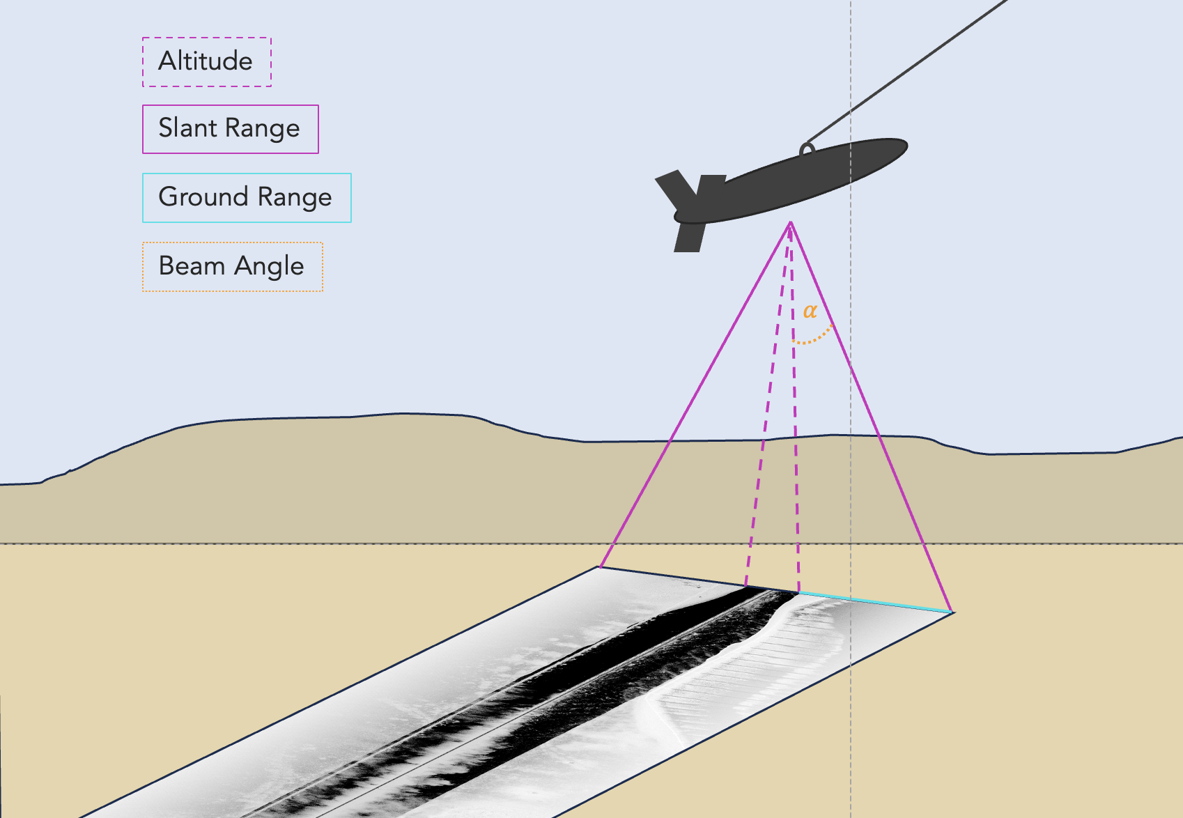
Slant range is the direct line-of-sight between the transducer and the seafloor. It is derived from the two-way travel time of an acoustic pulse from the transducer to the sea floor and back. Hence, slant ranges of neighbouring samples are very similar close to nadir where travel times are per se short, whereas at far distance from the transducer, they become significantly different. This change in range across the swath leads to perspective distortions by the slanted view: Two objects with mutual distance seem closer to each other at far range than two object with the same mutual distance that are at close range. Assuming a flat sea floor, the true ground distance can be derived using trigonometry as shown in Section 3.3.2 and Fig. 1 (Lurton, 2010) and (Blondel, 2009) . This requires the concept of bottom detection which will be explain further in Section 3.3.1.

2.1.3 Radiometric corrections

Radiometric correction addresses signal variation, attenuation and reverberation effects that occur when acoustic waves travel through water. Signal variation depends on various factors like distance, wave motion, beam pattern and instrument motion. More distant objects have weaker backscatter returns than objects closer to the transducer due to lower incidence angles and larger travel distances.

The typical antenna directivity pattern for a two-sided sonar device has a main lobe at around 45° with the main energy being emitted at around 35–65° (Chang et al., 2010). Side lobes with weaker signal strength usually also exist and need to be considered. Beam incidence angles can be calculated from phase shifts of the return signal that occur due to the speed of an object relative to the sensor. The effect of distance-related signal loss is compensated by applying Time Varying Gain (TVG) (Lurton, 2010). This mostly already happens during data acquisition inside the sonar hardware as a function of travel time and frequency. Motion of the sonar instrument (e.g. due to waves, differences in platform speed etc.) but also insufficient TVG can be the source of changes of ping energy that result in intensity patterns (e.g. stripes) along the track line. All of the above are systematic errors which can be corrected using statistics on beam pattern, distance from sonar and ping energy level normalisation. These corrections and other optional data processing steps are described in Section 3.4.

2.1.4 Georeferencing

Georeferencing is the process of adding geospatial information to a dataset, which in this case means transferring relative image coordinates to real-world coordinates (e.g. longitude/latitudes or coordinates in a projected reference system like Universal Transverse Mercator (UTM)). At this stage layback, the offset between the transducer and the GPS antenna, has to be taken into account and compensated. On a ping-by-ping basis, the centre (nadir) coordinates along with the outer swath edge coordinates and the sample size are used to form an evenly spaced grid with coordinates for each data sample. Sample in this case refers to slant range corrected backscatter value. The backscatter values are then mapped onto this grid using interpolation techniques. Coordinates of the inner swath and at the outer edges are calculated based on the ground range as described in Sections 3.3.1 and 3.3.2 (Lurton, 2010; Blondel, 2009). This approach becomes less accurate if bathymetry is varying laterally. If additional information about bathymetry is available, the sidescan mosaics can be fit to a more precise location by co-registering objects in the sidescan data with sea floor features on the bathymetry. However, this functionality is not implemented in SidescanTools. Conclusively, the georeferenced data from single files may be merged into one mosaic.

3 SidescanTools

SidescanTools is open-source, written in Python and uses some external libraries. The GitHub project includes a requirements.yml file to make installation via Anaconda easy (Anaconda, 2025).

The tool has been developed for full processing of data from commercial sidescan sonars. The aim is to apply geometric and radiometric corrections, to overall enhance image quality and to generate georeferenced images with user defined parameters on an easy-to-use graphical interface. As an alternative for advanced users who need to run SidescanTools on a system without UI (e.g. for deployment on AUVs or to save memory) the tool can also be used via a command line interface (CLI). In both cases, settings and parameters are stored and read from a configuration file project_info.yml. The implemented processing steps are explained in the following.

3.1 Design principles

The development of SidescanTools follows several key principles:

• 1. Open-source: SidescanTools is freely available and open-source under GPLv3 license, mainly targeted at NGOs or private people who use sidescan sonars and need to process and plot data.
  2. Modularity: The software is designed with a modular architecture that allows for easy extension and customisation of functionalities, e.g. headless operation for near real time use e.g. on AUVs.
  3. User-friendliness: SidescanTools aims to maintain an intuitive interface with focus on functionality and performance.
  4. Compatibility: Support for open and cross-platform data formats aims for a broad applicability across different sonar systems and manufacturers.

3.2 Supported data formats

SidescanTools supports two primary open data formats:

1. 1. JSF: An open file format developed by Edgetech, widely used in the marine industry. This file format has been decoded according to the official Edgetech documentation (Edgetech, 2025). Note that the format may be subject to future changes and unexpected errors may occur if the input file doesn’t meet the decoded format.
   2. XTF: A cross-platform readable file format that serves as a common standard for sonar data. It consists of several packets each delivered with an own header, which makes it a highly versatile file format (Kermarrec et al., 2020; Blondel, 2009). The XTF format is particularly useful because almost any raw sonar data format can be converted to XTF.

3.3 Key features and functionalities

The following sections describe how the previously mentioned processing steps for geometric and radiometric corrections, removal of noise and artifacts, image quality enhancement and the generation of georeferenced images are implemented in SidescanTools.

3.3.1 Bottom detection

Accurately identifying the sea floor in sonar data is crucial for subsequent processing steps and has to be done manually if no altitude/depth information is available. Usually, the bottom line is associated with the first bottom return, which is the first echo that the sonar receives from the bottom. In some cases, for example if sea grass or high obstacles (boulders, wrecks) that do not represent the true sea floor, are present, these would falsely be declared as first returns by most automatic edge detection algorithms. Here, the bottom line must be manually adjusted to the true bottom by the user. In SidescanTools, this is implemented as follows:

1. Chunk-based data presentation: The data are divided into chunks and visualised on the graphical user interface. Several common image adjustments like different colour palettes, hue, saturation, contrast and zoom levels are available to the user.
2. Threshold based detection: An algorithm with user-defined threshold is applied to convert the sidescan image into a binary mask which discriminates water column and ground pixels. On this masked image, an edge detection algorithm is deployed to find the most probable edge in the resulting binary image. This is done by finding all edges in the image and evaluating which edge is the most probable bottom line, which must preferably go through the whole image from top to bottom and have only ground pixels below itself. The threshold can be adjusted for each data chunk individually. This can be helpful for surveys with changing altitudes where different thresholds are required to correctly differentiate between water column and ground. Usually, starboard and portside lines are merged to find a common bottom line for both sides. In most cases, this is the best strategy because the nadir angle is small and thus neglectable, hence the bottom line is assumed to represent the sonar altitude. If this assumption does not hold for some specific cases, different strategies e.g. to separate the starboard and portside edge detection results can be selected.
3. Manual mode: To adjust falsely detected bottom lines, users can adjust the bottom line by drag-clicking on the chunk at the correct position. In the background, the bottom line is an array that masks the data array and is updated by the user’s input and saved for later processing steps.

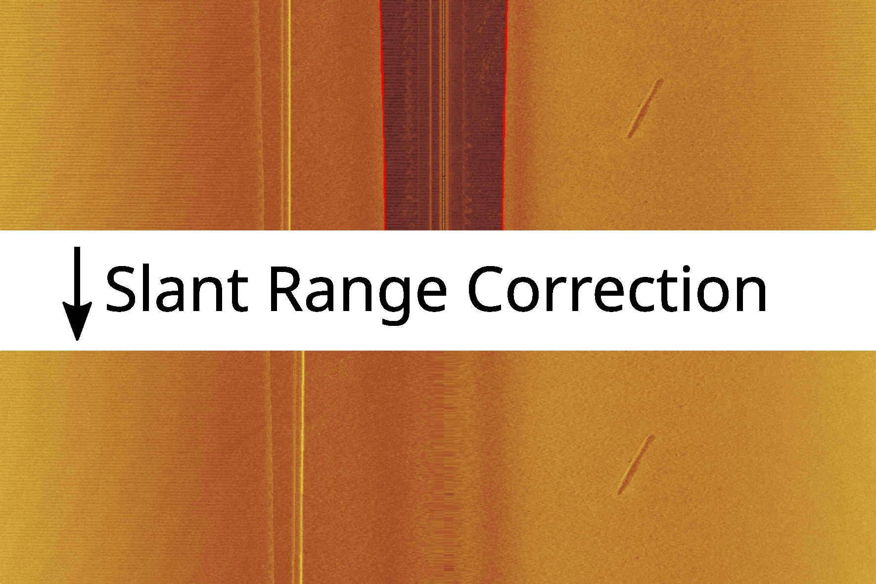
3.3.2 Geometric correction: slant range correction

Commonly, slant range correction is applied at this stage, using information of the detected bottom line from the previous step to remove the water column and to relocate the measured backscatter values across track. This correction is essential for accurate representation of ground distances and object sizes in the final image. The data are thereby projected onto a flat-assumed, horizontal sea floor. The assumption of a flat sea floor is required, because sidescan sonar measurements do not provide any additional information about across track water depths. Slant range correction is essential for accurate representation of ground distances and object sizes in the final image. The slant correction works by calculating the true ground distance for each sample with index i across the track as the hypotenuse of the triangle that is formed by nadir depth and the horizontal distance on ground d (Fig. 2; Blondel, 2009).

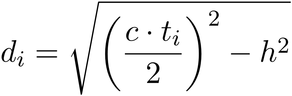(1)

where 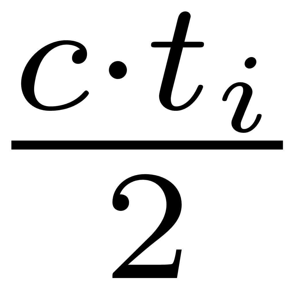 is the slant range at sample index i at time t, c is local speed of sound in water and h the local height above ground.

The result is a non-uniform vector of intensities for each ping that needs to be placed into a uniformly sampled vector of maximum original resolution. This introduces across track gaps which are then filled by linear interpolation of the entire vector. Often, the nadir angle of a sonar is not known and therefore assumed to be 0°. This is not problematic in most cases but leads to a small number of samples at close range which causes single intensities being stretched over multiple indices – a phenomenon that is often observed in processed sidescan data. The sonar is “blind” in these areas at close range.

3.4 Radiometric corrections

Radiometric corrections encompass downsampling of the data, removal of noise and artifacts and the correction of intensity gains to make objects appear with constant brightness across track, independent of their distance to the sonar.

3.4.1 Downsampling of data

If the raw sidescan data have significantly higher resolution – that is, they contain more samples per ping than required by the user, the resolution can be reduced by downsampling the data. Although this process results in some loss of information, the discarded data is often redundant and can be safely omitted to enable faster processing and reduce memory usage (Crochiere & Rabiner, 1983). In SidescanTools, this is implemented using SciPy’s decimate function, which downsamples each ping signal individually by an integer factor (SciPy community, 2025).

3.4.2 Removal of artifacts: Pie-Slice filter

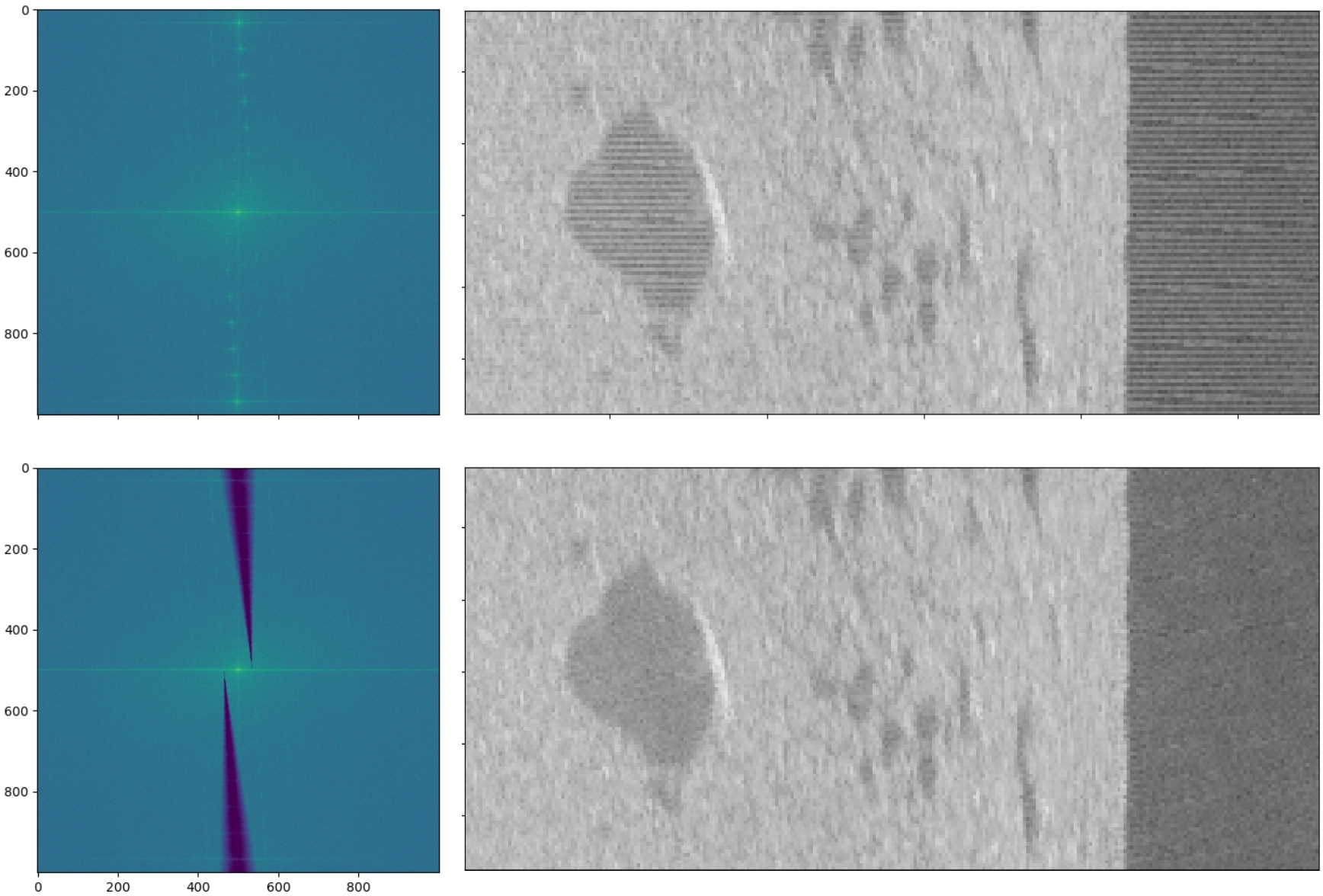
A Pie Slice filter can be used to remove stripy noise and artifacts (Wilken et al., 2012). The following implementation of this filtering approach is completely based on their work. These artifacts are usually visible in the sonar image as horizontal parallel stripes that are potentially tilted (Fig. 3). Often, the source is not known and noise artifacts may be caused by incorrect internal beam pattern correction, roll movements of the sensor, impact of waves, interference with other systems or electronic noise. To apply the pie slice filter, the data are separated into chunks of equal dimensions and transformed to the spectral domain by a two-dimensional fast Fourier transform (2D-FFT). In the spectrum, noise stripes become visible as spots of high energy that lie on a tilted line.

To remove these artifacts, the position of the bright spots is analysed in a first step. A straight line is then fitted through the centres of these spots to find the tilted axis on which the source of these artifacts is located. This line serves as the centre line for suppressing the spectral amplitudes, on which an attenuation of up to 80 dB is applied. To prevent an introduction of new artifacts by this filter, the suppression is applied in x-direction as a fading function to prevent sharp edges in the spectrum. Because the spots usually become more spread in their y-positions towards the outer edges of the image, the suppression itself is widened in y-direction. This is what gives the algorithm its name, because it looks like pie slices in a spectrum (Fig. 3). The slices are then rotated to fit between the points which shall be suppressed. As a last step, the spectrum is transformed back into the time domain. In SidescanTools, the width of the filter and the maximum attenuation are chosen to be 0.05 and 80 dB. These default values perform well in all situations that the authors encountered and should therefore also work for unknown sonar devices.

3.4.3 Gain normalisation: BAC and EGN

Gain normalisation equalises the return signal such that that the image appears with consistent brightness regardless of its distance or angle from the sonar. This also compensates for signal dispersion and attenuation over longer ranges, making distant objects more visible. Although most sonars apply a time-varying gain during data acquisition to amplify signals at greater distances, this built-in correction is not always optimal. Therefore, applying gain normalisation as an additional step helps to improve the overall image quality. SidescanTools offers two algorithms for this task which can be selected by the user depending on the amount of available data. Both are black-box approaches, meaning they only work on observed values and have no information about the sonar system and its parameters. It is however important to note that the type of seafloor plays a crucial role for the relationship between incidence angle and backscatter amplitude. The below described methods for gain normalisation cannot entirely account for changes in geomorphology during a survey. It is recommended to start a new survey file every time a geomorphological boundary crossed. Empirical gain normalisation (EGN) tables can then be calculated for the different geomorphological realms.

Beam angle correction

To compensate for angle-dependant signal attenuation, the beam angle correction (BAC) algorithm estimates the beam pattern of the sonar device from the recorded data. This algorithm only takes data of the currently processed file into account and returns good results if little data are provided. If more data are available, the more sophisticated EGN (see next section) method would yield better results. When applying BAC, the incidence angle to the sonar is calculated for each sample of each ping for the current recording. All samples of the same angle are then averaged to get an estimated beam pattern. This is used to adjust the intensities of each sample across all pings. This approach is independent of the distance to the ground and therefore needs only little data to work (Chang et al., 2010):

s'(ꞷ,r) = s(ꞷ,r) · B(ꞷ) (2)

The correction table for BAC is defined with the above Eq. 2, where , ꞷ, r: beam angle/range and Nꞷ: number of samples with the same beam angle.

Empirical gain normalisation (EGN)

EGN is an empirical method to estimate the sonar beam pattern and depends, contrary to BAC, on both range and angle:

s'(ꞷ,r) = s(ꞷ,r) · B(ꞷ,r) (3)

The correction table for EGN is defined with the above Eq. 3, where , ꞷ beam angle, r: range and Nꞷ: number of samples with the same beam angle and range.

Note the additional range dependency of B(ꞷ,r) and Nꞷ,r for EGN which is different to BAC.

Based on statistical analysis, an EGN table is created which can be used to normalise the intensity of the backscatter values. This correction table can be applied to all sidescan data that have been recorded with the same device (Blondel, 2009).

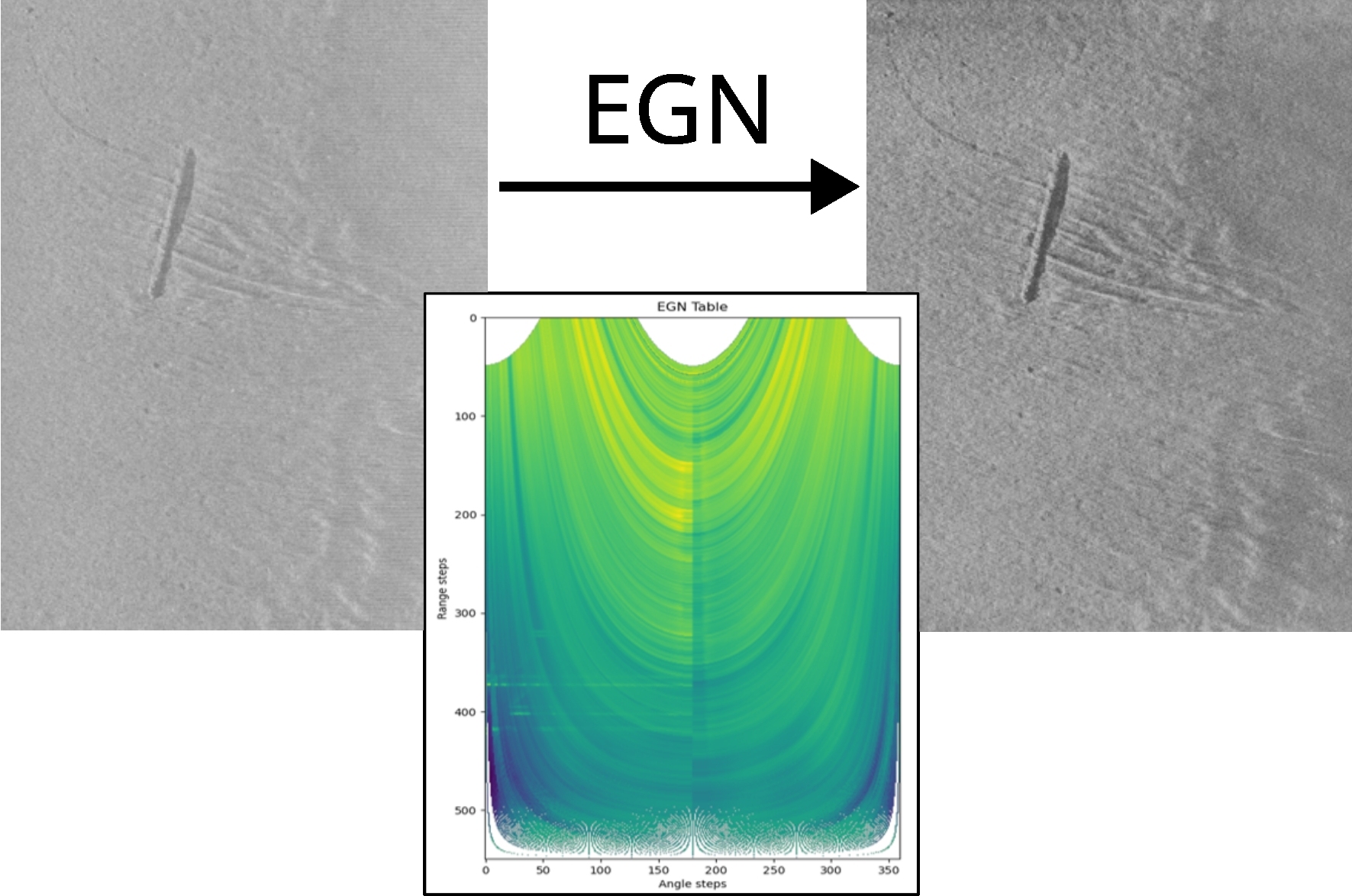
At first the EGN table is calculated by binning all backscatter values depending on their incident angle and ground range. At this stage, all recordings from all files imported into the current project are included. The project should therefore contain only data from a survey of one specific sonar system. The result is a matrix of binned values with the average calculated for each bin. The resulting table is a matrix of bins in which each bin contains the average of its assigned values.

Provided that sufficient data are present, the mean value of each bin now represents the transmitted energy from the sonar and has thus become independent from any reflecting objects or other ground returns. The inversion of this matrix yields the so called EGN Table and is used to normalise all backscatter intensities depending on their angle and range of the current dataset (Fig. 4). It also may be used for later recordings of the same sonar system.

The user should keep in mind that this method only works for an individual instrument and only if sufficient data are available. If unsure, it is safer to use BAC.

3.5 Post-processing

To further improve the quality of the resulting images, additional filters can be applied like sharpening or Contrast Limited Adaptive Histogram Equalization (CLAHE). This is useful to make objects stand out more from the background and to improve the performance of object detection methods.

3.5.1 Sharpening filter

Image sharpening can be implemented by enhancing the contrast with a homomorphic filter. The concept is to design a filtering function that can operate on the illumination and reflectance components of the image separately (Gonzalez & Woods, 2001). The illumination component of the image is influenced by slow spatial changes and is therefore displayed by the low frequency components in both dimensions of the 2D-spectrum. In contrast, the reflectance component tends to vary more abruptly, especially at the edges of objects, and is therefore more present in the high frequency components of the 2D-spectrum. These associations are only rough approximations, but they can be used to achieve an overall sharper image.

To control the ratio of illumination and reflectance, a two-dimensional symmetric filter is designed to attenuate low frequencies and enhance high frequency components of the image.

3.5.2 Contrast limited adaptive histogram equalization

Adaptive Histogram Equalization (AHE) is a commonly used image processing technique to enhance contrast. It is called adaptive, because it calculates several histograms, each for a specific region of the image, and redistributes the lightness values of each region. This achieves an improved local contrast and sharper definitions of edges of objects in each region. Because of the nature of sidescan images, there are often regions of nearly constant intensities. Since the histogram of such regions is highly concentrated, AHE tends to overamplify the contrast in these regions. This also causes overamplification of noise and makes the resulting image look grainy. To avoid this, CLAHE is used here. This works by clipping the region histograms at a user defined threshold to reduce the problem of noise amplification. For more information about the working principle of CLAHE, please refer to (Zuiderveld, 1994).

4 Georeferenced image export

Georeferencing is the process of mapping image coordinates to global coordinates. The following section describes how these steps are implemented in SidescanTools.

4.1 Navigation pre-processing

To create a coherent georeferenced image, the raw navigation data are pre-processed in several steps:

1. 1. Remove duplicates: If duplicate coordinates are present e.g. due to poor GNSS quality, these are removed. The remaining unique coordinates are stored in a separate array, referred to as ‘unique arrays’ (one per channel).
   2. Interpolate and fit to original length: As the unique arrays are usually shorter than their originals (because duplicates have been removed), they are interpolated using the cubic b-spline method from scipy interpolate package (Virtanen et al., 2020). To re-gain full array length and maintain the true number of pings, the interpolated coordinates are evaluated on the ping sequence of original length. The resulting array is referred to as ‘uniformed ping array’.
   3. Smooth track: The interpolated coordinates are smoothed using a Savitzky-Golay filter as implemented in scipy (Savitzky, 1964). This filter preserves trends and reduces sharp peaks by fitting low-order polynomials to the data with a moving window. A window size of 100 pings and a polynomial order of two has proven to be a good choice between preserving local tendencies and at the same time avoiding large jumps in the data.
   4. Course over Ground (CoG): To derive correct outer swath coordinates later on, course over ground or bearing angle is needed. This is calculated using the arctan of the distances between the current ith and the following (i+1)th ping position of the smoothed and interpolated track:
      
      

      θ(i)=tan-1(dxi,dyi) (4)

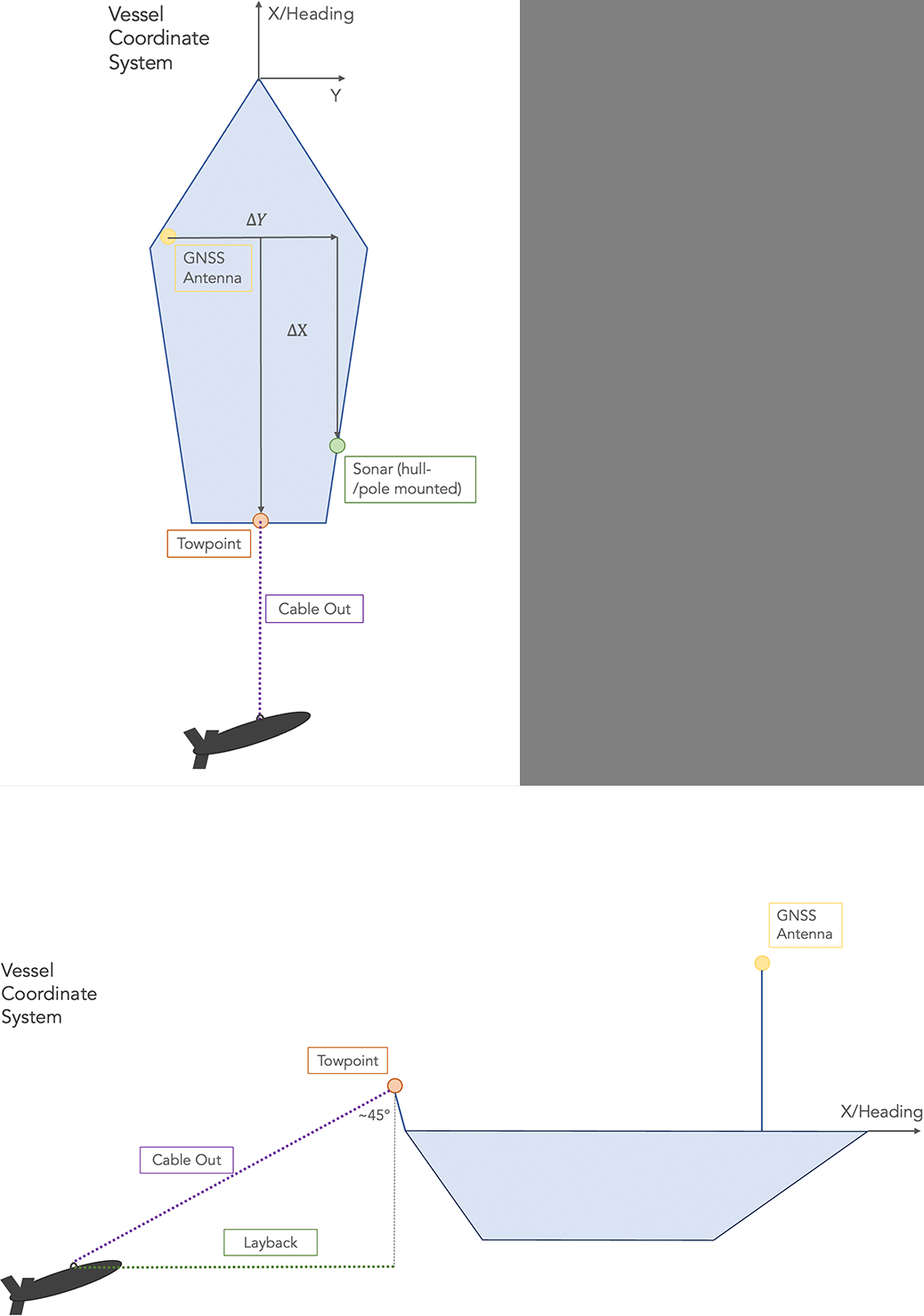
      where θ is the course angle, (dxi,dyi) represent the distances between the ith and the (i+1)th coordinate
   5. Offsets: If not already implemented via the acquisition software, SidescanTools offers the user to add offsets between the GNSS antenna and the sonar transducer as well as a cable out length, if the sonar has been towed. The vessel coordinate system is shown in (Fig. 5). X is positive in forward direction of the ship from the GNSS antenna position, Y is positive to the right side of the ship from the GNSS antenna position. Negative X/Y values indicate that the sonar is located behind/left of the GNSS antenna. If the sonar is towed and the layback has not been implemented prior to the survey, the user can enter a cable length, which is converted to layback assuming a rope angle of 45° at the towpoint. This method cannot account for layback changes due to currents or drift. It is assumed to be static, which in reality is true only if there is no current.

Note that in early development raw heading values were used to calculate outer swath coordinates. This led to inaccuracies due to drift and water current which is why it has been replaced by the calculated course over ground.

4.2 Determination of outer edge coordinates

Sonar data are provided as a time-series of consecutive pings and only the centre (nadir) coordinates are known from the raw data. Inner-swath and outer edge coordinates can be determined using ground range and course angle information:

1. Outer edge coordinates: Longitudes and latitudes must first be converted into a metric coordinate system (here Universal Transfer Mercator, UTM). The outer swath coordinates can then be calculated like so:
   Backbord
   Nout = Nnad – g·cosθ (5)
   Eout = Enad + g·sinθ
   
   Starbord
   Nout = Nnad – g·cosθ (6)
   Eout = Enad + g·sinθ
   where Nout/nad / Eout/nad represent the outer/nadir Northing/Easting coordinates, respectively, g is the ground range, θ is the course angle.
2. For later use, the computed UTM coordinates are converted back to longitudes and latitudes.
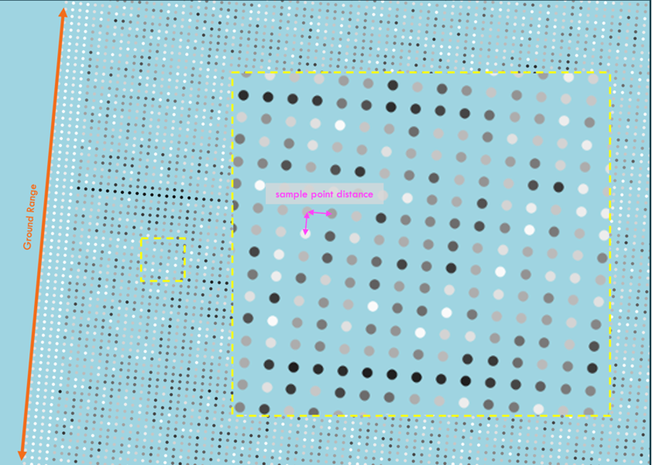
3. To obtain coordinates for each individual sample, an evenly spaced raster of coordinates is now formed between the nadir and outer edge. The resolution of the raster is determined by dividing the ground range by the number of samples, which at the same time represents the finest possible pixel resolution of the data (Fig. 6).

4.3 Mapping data to raster

4.3.1 Creating XY array

The arrays of interpolated, regularly spaced sample coordinates are written to a table which can optionally be exported to disk to investigate navigation. This table will be used in the next step to map the backscatter values on.

4.3.2 Generate output raster

The output raster generation is mainly accomplished with Generic Mapping Tools (GMT) (Wessel et al., 2019). Firstly, the previously created coordinate raster is concatenated with the backscatter data to obtain an xyBs (longitude, latitude, backscatter) data array. This serves as input to a GMT nearneighbor algorithm which maps the backscatter values on the coordinate raster. Optionally, to reduce noise and data size, a GMT block-median can be applied prior to the nearneighbor gridding. The following parameters are necessary:

1. 1. Region: Describes the bounding box of the data to be processed and is automatically derived with the gmtinfo command. The coordinate precision, which defines the accuracy of the size of the region bounding box, is based on the number of decimal places of the coordinates. This is to select an optimal bounding box size, to reduce computing time.
   2. Resolution: The resolution is typically user-defined and specifies the cell size of each pixel in the output grid. It can be adjusted in the UI.
   3. Search radius: The nearneighbour algorithm additionally needs a search radius parameter, which specifies the number of neighbours around a grid cell that the algorithm includes to calculate the cell’s interpolated value. This is also user defined, but if unsure, double the resolution value usually yields good results.
   4. Clip backscatter values to range: As the output image data can only have values between 0-255, the output raster is clipped to this range using xarray package (Hoyer, 2017). Minimum/maximum values will be replaced by ‘0’/’255’, respectively. This ensures to avoid empty cells with unreasonably low/high numbers.
   5. Assign CRS: So far, there is no information about a coordinate system and/or geodetic projection yet. This is assigned using rioxarray package and set to EPSG:4326/WGS 84 with rioxarray.set_crs. Optionally, if the UTM export option is selected by the user, the dataset is reprojected to the respective UTM Zone with rioxarray.reproject.
   6. Export: The final raster is exported as a compressed Geotiff with rioxarray.to_raster.

5 Discussion and outlook

SidescanTools is designed for an easy workflow to process sidescan data and export geo-referenced images. It is less extensive in functionality compared to other popular commercial software packages, which is mainly due to restricted data formats.

It is further known that some loss of metadata happens when converting proprietary raw data formats to the cross-platform XTF format. Due to these limitations, we can only work with the available metadata which might result in inaccuracies. Furthermore, SidescanTools was originally developed to process data from a pole-mounted Starfish device used with poor quality GPS and without attitude information. Although we tried to take common error sources into account, the (navigation) pre-processing has been tailored to the need of reducing errors of this specific setup. Data from other devices may contain other error sources that potentially have not been taken care of yet.

SidescanTools is also available as a CLI version for head-less use e.g. on AUVs during dives. This enables the data to be processed online without requiring the AUV to be retrieved and may be useful for diving operations where the AUV must be able to alter its course spontaneously and based on ‘what it sees’ to target specific objects. This procedure has been successfully run in a first field test.

SidescanTools is still in active development, but has reached a feature range that makes it well usable for sidescan data processing. As it is an open-source alternative it has potential to grow with increasing user numbers. We rely on a community for feedback about lacks, additional or missing features and general suggestions for improvement. Issue reporting or feature requests can be submitted directly in the git repository (https://github.com/sonoware/sidescantools/issues).

References

Anaconda (2025). Anaconda. Anaconda Inc., Austin, USA. https://anaconda.org/ (last accessed 10 November 2025).

Blondel, P. (2009). The Handbook of Sidescan Sonar. Chichester: Praxis Publishing Ltd.

Bruns, I., Holler, P., Capperucci, R. M., Papenmeier, S. and Bartholomä, A. (2020). Identifying Trawl Marks in North Sea Sediments. Geosciences, 10(11), 422. https://doi.org/10.3390/geosciences10110422

BSH (2016). Guideline for Seafloor Mapping in German Marine Waters Using High-Resolution Sonars (1^st ed.). Federal Maritime and Hydrographic Agency, Hamburg/Rostock, Germany. https://www.bsh.de/download/Guideline-for-Seafloor-Mapping.pdf (last accessed 25 March 2026).

Chang, Y.-C., Hsu, S.-K. and Tsai, C.-H. (2010). Sidescan sonar image processing: Correcting brightness variation and patching gaps. Journal of Marine Science and Technology, 18. https://doi.org/10.51400/2709-6998.1935

Crochiere, R. and Rabiner, L. (1983). Multirate Digital Signal Processing (2^nd ed.). Englewood Cliffs: NJ: Prentice-Hall.

Díaz-Mendoza, G. A., Krämer, K., von Rönn, G. A., Schwarzer, K., Heinrich, C., Reimers, H.-C. and Winter, C. (2023). Circular structures on the seabed: differentiating between natural and anthropogenic origins—Examples from the Southwestern Baltic Sea. Front. Earth Sci., 11:1170787. https://doi.org/10.3389/feart.2023.1170787

Díaz-Mendoza, G. A., Krämer, K., von Rönn, G., Heinrich, C., Schwarzer, K., Reimers, H. C. and Winter, C. (2024). Hotspots of human impact on the seafloor in the Southwestern Baltic Sea. Continental Shelf Research.

Edgetech (2025). JSF File and Message descriptions (Rev P, 11.09.2025). https://www.edgetech.com/wp-content/uploads/2023/04/0023492_Rev_P.pdf (last accessed 7 November 2025).

Gonzalez, R. C. and Woods, R. E. (2001). Digital Image Processing (2^nd ed.). Upper Saddle River, New Jersey : Prentice-Hall, Inc.

Grządziel, A. (2023). The Impact of Side-Scan Sonar Resolution and Acoustic Shadow Phenomenon on the Quality of Sonar Imagery and Data Interpretation Capabilities. Remote Sensing, 15(23), 5599. https://doi.org/10.3390/rs15235599

Hoyer, S. H. (2017). xarray: N-D labeled Arrays and Datasets in Python. Journal of Open Research Software, 5(1), 10.

Kermarrec, E., Saman, L. and Tauvry, S. (2020). eXtended Triton Format (XTF): File format specification (Rev. 42). https://www.ecagroup.com/en/xtf-file-format (last accessed 25 March 2026).

Lurton, X. (2010). An Introduction to Underwater Acoustics (2^nd ed.). Heidelberg: Springer Berlin.

Marx, D., Feldens, A., Papenmeier, S., Feldens, P., Darr, A., Zettler, M. L., Heinicke, K. (2023). Habitats and Biotopes in the German Baltic Sea. Biology, 13(1), 6. https://doi.org/10.3390/biology13010006

Savitzky, A. M. (1964). Smoothing and Differentiation of Data by Simplified Least Squares Procedures. Analytical Chemistry, 36(8), 1627–1639.

SciPy community (2025). scipy.signal.decimate. https://docs.scipy.org/doc/scipy/reference/generated/scipy.signal.decimate.html (last accessed 7 November 2025).

Virtanen, P., Gommers, R., Oliphant, T. E., Haberland, M., Reddy, T., Cournapeau, D., Burovski, E., Peterson, P., Weckesser, W., Bright, J., van der Walt, S. J., Brett, M., Wilson, J., Millman, K. J., Mayorov, N., Nelson, A. R. J., Jones, E., Kern, R., Larson, E., et al. (2020). SciPy 1.0: fundamental algorithms for scientific computing in Python. Nature Methods, 17, Article 3. https://doi.org/10.1038/s41592-019-0686-2

Wessel, P., Luis, J. F., Uieda, L., Scharroo, R., Wobbe, F., Smith, W. H. F. and Tian, D. (2019). The Generic Mapping Tools version 6. Geochemistry, Geophysics, Geosystems, 20, 5556–5564. https://doi.org/10.1029/2019GC008515

Wilken, D., Feldens, P. and Wunderlich, T. (2012). Application of 2D Fourier filtering for elimination of stripe noise in side-scan sonar mosaics. Geo-Marine Letters, 32, 337–347. https://doi.org/https://doi.org/10.1007/s00367-012-0293-z

Zuiderveld, K. (1994). Contrast limited adaptive histogram equalization. In P. S. Heckbert (Ed.), Graphics gems IV (pp. 474–485). San Diego: Academic Press Professional, Inc.