


Preamble
This manuscript is a reprint of the original paper previously published in 1976 in The International Hydrographic Review (IHR, https://ihr.iho.int/): Eaton, R. M., Wells, D. E., and Stuifbergen, N. (1973). Satellite navigation in hydrography. The International Hydrographic Review, 53(1), 99–116. https://journals.lib.unb.ca/index.php/ihr/article/view/23736
“I’ll put a girdle round about the earth in forty minutes.”
(Puck in “Midsummer Night’s Dream” by William Shakespeare).
1 Introduction
Satellite Navigation (“Navsat”) is a remarkable development in positioning that gives a dozen or more good fixes per day, anywhere in the world. The accuracy of the ship’s position from a good pass is from 60–600 m, depending on how well the ship’s course and speed is measured. For stationary receivers, this positioning accuracy improves to about 20 m.
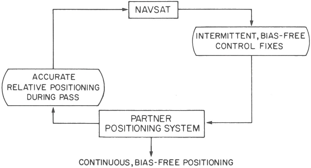
Navsat’s great value to hydrography is that the fix is virtually free of systematic position errors. Navsat is extremely useful in offshore surveys as a complementary partner to a high resolution, continuous system which has systematic biasses or which accumulates error with time; we describe integration with rho-rho (range measuring) Loran-C, and Doppler Sonar. The continuous system feeds accurate course and speed to Navsat, which in turn provides a control network of intermittent, bias-free fixes. By bridging a number of satellite fixes the combined system means out random errors and improves on the single-pass accuracy of Navsat.
Navsat has many auxiliary applications. It is used to resolve the cycle ambiguity in low frequency radio aids; to calibrate both marine survey positioning systems and radio aids to navigation; to position the transmitters for the radio aids; to position offshore drilling rigs; and as a geodetic instrument capable of establishing shore control to 1 m accuracy.
The “Datum Shift” between a Navsat position and a position from the local geodetic control often causes confusion. We outline the reason for the difference, and give algorithms for computing it.
2 The Navy Navigation Satellite System (NNSS)
“Transit” (i.e. satellites that pass overhead) is the specific name for this type of satellite system, but we will use the more usual term “Navigation Satellite” abbreviated to “Navsat”. Those who are not familiar with it should read Stansell (1968).
To recapitulate briefly, the satellites broadcast two stable, harmonically related carrier frequencies at 150 MHz and 400 MHz; as the satellite passes the ship, at 7.3 km/sec., the receiver measures the amount by which these stable frequencies are Doppler shifted. The satellites also transmit a series of digital signals, by imposing balanced phase modulations on the carriers. These signals can be used as time marks, and they contain parameters describing the satellite orbit. The parameters are computed by fitting orbital arcs to Doppler measurements from four tracking stations in Maine, Minnesota, California and Hawaii, and extrapolating the arc for 16 hours beyond the time of the last data used. These orbit predictions are injected into each satellite’s memory twice a day. There are at present six operational satellites in almost circular polar orbits having heights of 1100 km (compare with the earth’s radius of 6400 km) and periods of one hour and forty minutes (not forty minutes, as predicted by Puck; Shakespeare must have been using poetic licence!). Fig. 1 illustrates the configuration.
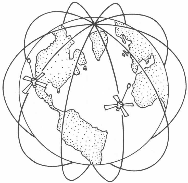
At 1100 km height the satellite can be received over a circle on the earth’s surface of radius 30°. All satellites transmit the same frequency, but because the Doppler shift is large (about 8 kHz) compared with receiver bandwidth, the transmissions from two satellites interfere only if the passes are nearly simultaneous. The satellites all pass over the pole, and so at the equator their orbits are well separated; simultaneous passes are rare at low latitudes, and there can be gaps of four hours between passes. At high latitudes simultaneous passes occur more frequently, but there are more passes available.
3 How the measurements are made
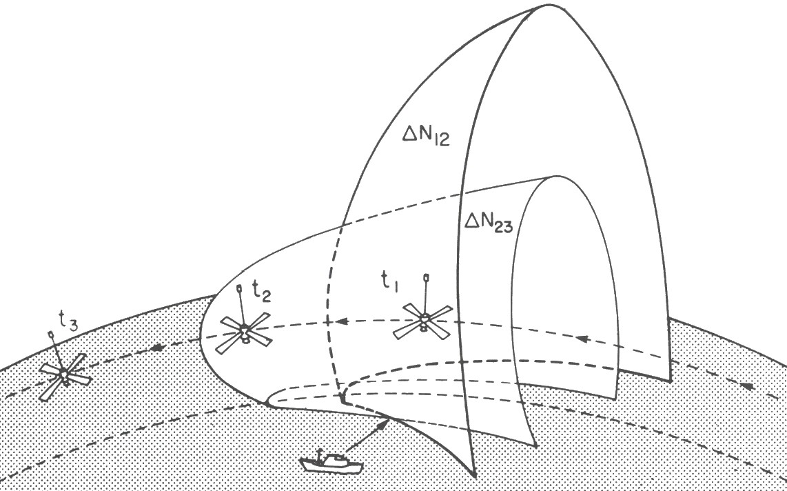
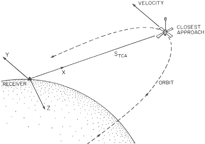
As in any other radio positioning method, the Navsat receiver makes measurements on transmissions from known points (in this case the known position of the satellite at given time intervals along the orbit) and translates these into position lines whose intersection defines the ship’s position. In Navsat the receiver measures Doppler counts by integrating the changing frequency as the satellite’s velocity relative to the receiver changes, and transforms these into differences of distance that define hyperboloids in space. These intersect each other and the earth’s surface at the ship (Fig. 2). Satnav is a hyperbolic radio aid in the sky.
Fig. 3 shows a satellite travelling at a speed of about 7.3 km/sec., continuously transmitting the frequency fg, a sequence of time marks represented by t1 , t2 , … t j, … and orbital data establishing its position at these times. The receiver has an oscillator generating the frequency fg .
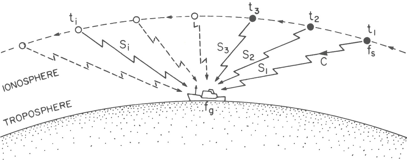
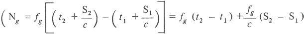
Each time mark transmitted by the satellite at t arrives at the ship after travel time Sj /c, where for the moment we assume the signals propagate in a vacuum. For example, between (t1 + S1 /c) and (t2 + S2 /c), the number of “satellite clock ticks” (or cycles of f arriving at the receiver must equal the number transmitted by the satellite, that is
| (1) |
However the number of “receiver clock ticks” (or cycles of fg) occurring during this same period is
 |
(2) |
The receiver actually measures “ticks” of the beat frequency between fg and fs (fs being deliberately offset 80 parts per million below fg to avoid negative cycle counting), so that the measured Doppler count is
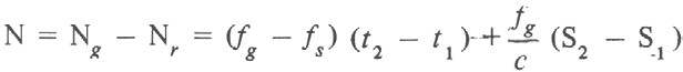 |
(3) |
In this equation we know the counting period (t2 – t1 ), the vacuum velocity c, and the satellite frequency fs, which is included with the orbital data, but we don’t know fg. The slant ranges Si depend on the known satellite positions and the unknown ship’s positions, at time (ti + Si /c).
Several assumptions buried in the derivation of Eq. 3 are:
- Signals propagate as in a vacuum.
- The orbital data establishes true satellite position at time t .
- Doppler counting starts precisely when a time mark arrives at the receiver’s antenna.
- Both fg and fS are constant during a pass.
- Relativistic effects are negligible.
For some applications, such as general navigation, all these assumptions are valid. For other applications, such as geodetic surveying, none of them are, and corrections must be made for each assumption. Currently for hydrographic surveying only the first assumption is corrected for.
4 How the fix is obtained
The satellite generates time marks every 20 ms, so that in principle a maximum of 45 000 Doppler counts could be measured during one pass (equivalent to 45 000 hyperbolic lines of position per fix). In practice, so much data would vastly increase computational problems without improving the results. In general we need only make enough measurements to ensure good redundance, and Doppler counts of 20 seconds (maximum 54 counts per pass) are generally measured, depending on the hardware and software being used.
In any case we end up with many more lines of position than we would need to fix a single ship’s position. However, the ship occupies a different position for each slant range Si in Eq. (3), so the paradox is that no matter how much data we collect during a pass it will not be sufficient to solve for all the ship’s positions, To overcome this problem, we must use an independent navigation system to construct a table of ship’s positions for each Si . This table of positions is then adjusted as a whole, together with the unknown fg , in a series of iterations, until the slant ranges calculated between ship’s position and satellite positions fit the slant range differences measured by the Doppler counts as well as possible. If the table of relative ship’s positions is distorted then this fit may be poor, and the adjusted table wrong. In fact, most often the table is constructed on the assumption that the ship’s course and speed are constant during the pass, limiting the usefulness of Navsat to passes during which these conditions are met. No matter how carefully constructed, error in the table of relative ship’s positions is the predominant factor in determining fix accuracy from moving ships.
5 Coordinate systems
In contrast to other radio positioning systems, Navsat operates in three dimensions rather than two dimensions. However it remains a two dimensional positioning system; only two coordinates can be obtained from a single pass. (Three dimensions can be obtained by combining data from several passes at a motionless receiver). Since we can determine only two coordinates from Navsat we must choose a value for the third coordinate ourselves. Usually the two coordinates we compute are latitude and longitude and the coordinate we specify is ellipsoid height. Errors in the choice of height will mainly affect the longitudes computed.
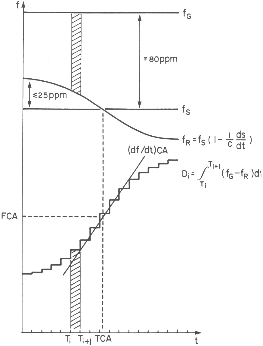
Some insight into the nature of a Navsat fix and how different errors affect fix accuracy can be gained by considering another two dimensional coordinate system, the Guier plane (Guier, 1965). To discover this coordinate system, we first look at the characteristics of a set of Doppler measurements (Fig. 4 and 5). The three parameters which most fully represent the information contained in such a set of measurements are the time at which the satellite most closely approaches the receiver tca, the frequency at closest approach fca, and the Doppler curve slope at closest approach (df/dt)catca measures the receiver position along the satellite track (since Transit satellites are in polar orbits, this along-track coordinate is equivalent to latitude). At closest approach the Doppler shift is zero and fca measures the frequency offset (fg – fS ). A less obvious relationship exists between the slope of the Doppler curve at closest approach (df/dt)ca and the minimum range Stca between satellite and receiver at that instant. Since the Doppler shift measures the relative velocity between satellite and receiver, then the slope of the Doppler curve measures relative acceleration. The closer the satellite trajectory is to the receiver (that is the smaller the closest approach range), then the greater the relative acceleration, and the steeper is (df/dt)ca Thus there are two geometrical properties of each pass, the along-track and cross-track (slant range) coordinate at closest approach, which, together with the frequency offset, best characterize the observed data. The Guier plane is the two dimensional coordinate system whose axes are the alongtrack and cross-track coordinates at the point of closest approach. It is unique to each satellite pass, and is tilted with respect to the receiver’s horizon plane by the closest approach pass elevation angle.
6 Accuracy of the fix
Let us consider the effects various errors will have on the Doppler curve, and hence the Guier plane coordinates.
Part of the signal path from the satellite lies through the ionosphere, part through the troposphere (Fig. 3). Uncorrected ionospheric refraction shortens satellite-to-receiver slant ranges, the net effect of which is to reduce the closest approach slant range (cross-track coordinate) by about 50 m.
Ionospheric refraction is frequency-dependent, and so can be corrected by combining Doppler measurements at the two measuring frequencies of 150 and 400 MHz, with residual errors of no more than a few metres.
Uncorrected tropospheric refraction increases the closest approach slant range by about 20 m. We can correct for tropospheric refraction using a model of the vertical profile of refractivity, and average or observed surface weather conditions. The residual range errors are 5 cm above 20° satellite elevation and 45 cm at 5° elevation. (Hopfield & Utterback, 1973). This tropospheric correction is not made by most Navsat fix programs, however they usually automatically eliminate measurements made below 7½° elevation, where the tropospheric effect is most serious.
Errors in satellite orbit coordinates affect both along-track and cross-track coordinates. However, the main source of orbit errors is unpredictable atmospheric drag effects, so the along-track effect (30 m) predominates. Signal delays in the receiver affect the along-track coordinate by 10 m. Oscillator drift affects the Doppler curve slope, and thus the cross-track coordinate by about 1 m. An error in along-track (North-South) ship’s velocity affects the Doppler curve slope and thus the cross-track coordinate. The time of closest approach is midway between the two “shoulders” of the Doppler curve; asymmetric data which does not contain equal portions of both shoulders weakens the determination of t , and hence the along-track coordinate.
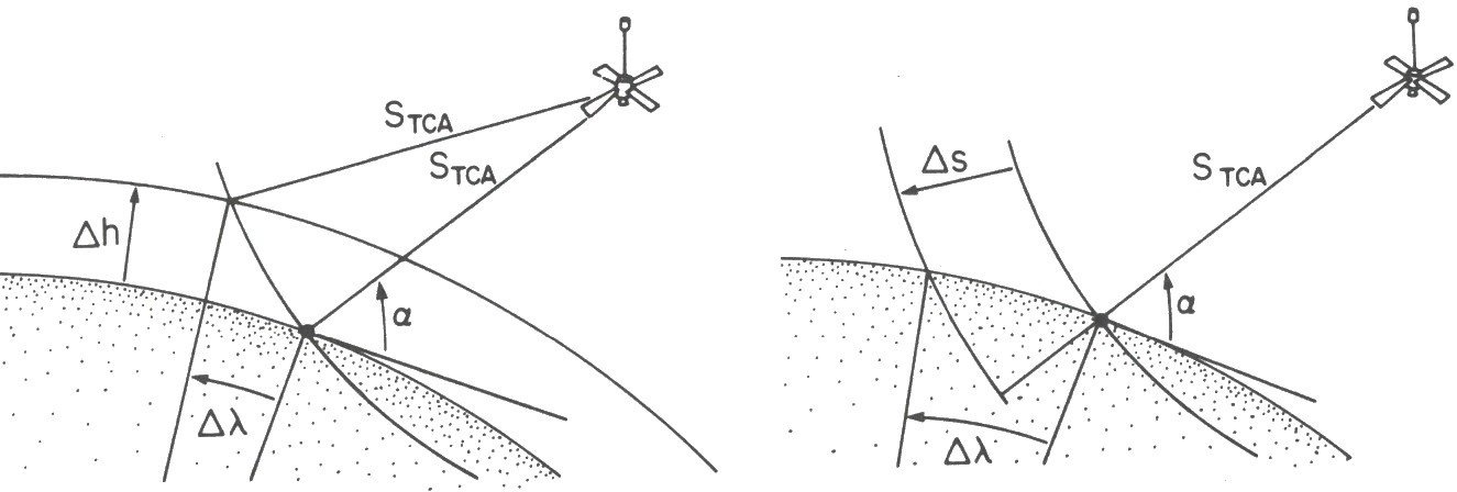
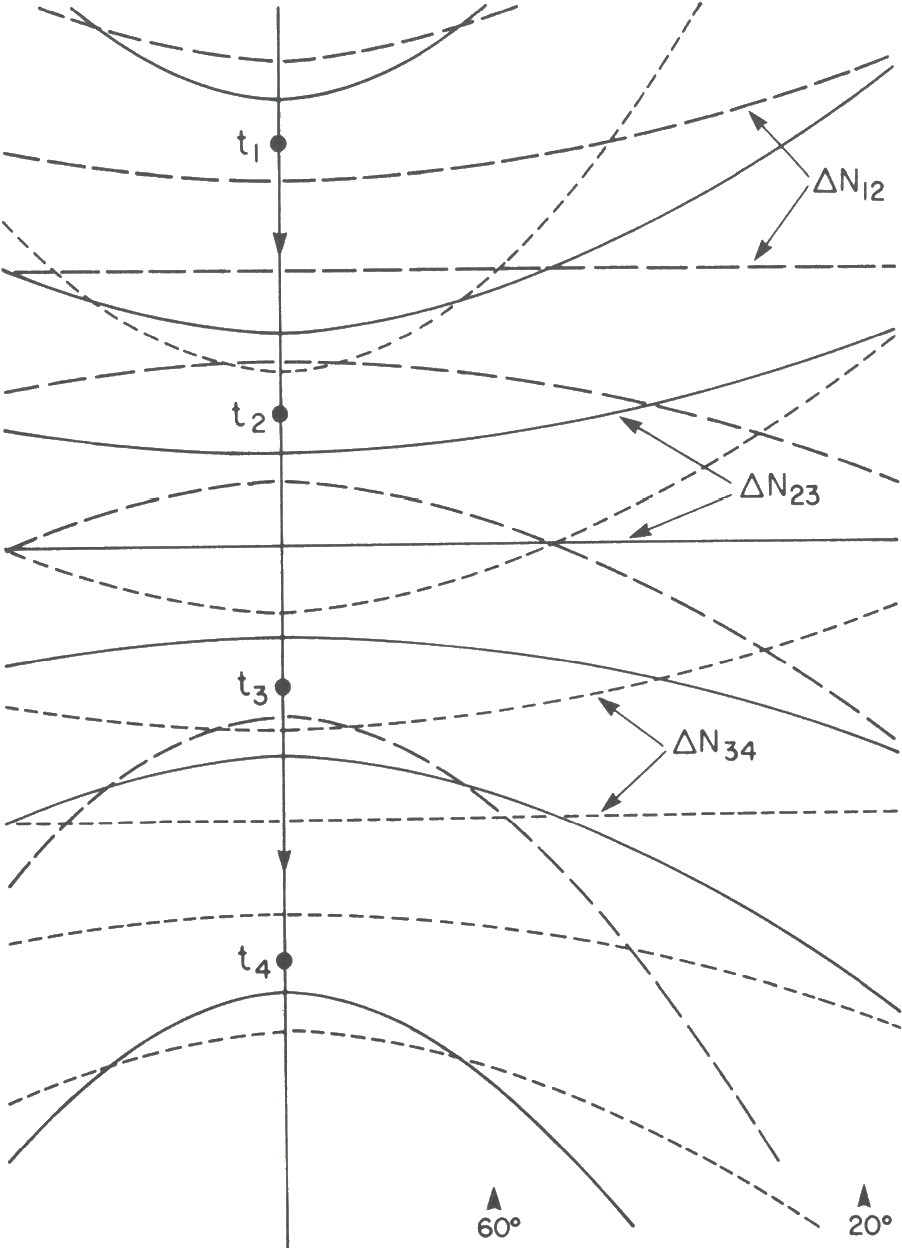
While we do not usually compute our position in the Guier plane, the results we obtain are equivalent to navigating in the Guier plane (extracting the essential information from the pass), and then transforming lo a more conventional coordinate system, such as latitude, longitude and height. This transformation would simply consist of rotating the Guier plane through the pass elevation angle into the horizon plane. Latitude corresponds to the along track coordinate. Longitude and height are both functions of the Guier plane cross-track coordinate and the pass elevation angle, and are therefore not independent. Navigating in the horizon plane, we must hold the height fixed, and consequently height errors will affect longitude. The cross-track errors are not strongly dependent on pass elevation, however on transformation to Latitude and Longitude coordinates a small cross-track error becomes a large longitude error for high elevation passes. Fig. 6 illustrates this.
Fig. 7 shows a different approach to Navsat error analysis, by looking at the position lines generated on the earth’s surface by a series of Doppler counts.
7 Fix accuracy diagnostics
A number of diagnostics can be used to indicate the quality of a particular satellite fix. Most important is that enough Doppler measurements be made. Using 30-second Dopplers as an example, if less than 20 counts are measured (after rejecting the low elevation data) the reason may be any one of low elevation pass, low signal level, interference, poor antenna site, or poor receiver performance. Regardless of the reason, the resulting fix will probably be poor.
As mentioned above, the accuracy of a fix in latitude and longitude coordinates depends strongly on the pass elevation angle. For high elevation passes (greater than 60°) the longitude is poorly determined. For low elevation passes (less than 20°) refraction and the shallowness of the Doppler curve degrade the fix accuracy.
Maintaining a plot of the computed values for the local oscillator frequency, fg , as a function of time provides a sensitive indicator of potential fix errors. The frequency fg should change slowly and linearly with time (a few parts in 1010 per day for the best oscillators). An outlying value of fg indicates that something is wrong (very often the ship’s relative motion input) and the probability of a poor fix is high. However maintaining a record of fg is difficult with most current fix programs, since they compute (fg – fS), not fg ; and fS is different for each satellite. Separate plots for each satellite can be maintained, or the value for can be located in the orbital message data and f computed manually.
A fourth diagnostic is the “residual” value provided by many fix programs. The residual expresses the fit between the computed slant range difference (based on the final ship’s coordinates) and the measured slant range differences (based on the measured Doppler counts); the lower the residual the better the fit. A poor fit is unlikely to give a good fix, but the converse is not necessarily true. Caution should be used in comparing residuals between different programs. Every measurement provides a residual, which can be expressed either in metres (slant range difference) or Doppler counts. The single “residual” value printed out may be the largest residual, or the RMS value of the residuals, or the mean of the absolute values of the residuals.
Other diagnostics are the number of iterations a pass required to converge, the symmetry of the data about closest approach, and, for some receivers, a digital representation of the signal strength.
Despite all these diagnostics, an undetectable “wild” fix will occasionally occur which satisfies all the diagnostic criteria, except that the position is very much in error. For this reason it is never safe to blindly force other navigational systems to agree with Navsat positions.
8 Accuracy at sea
We have outlined the size of errors that can be contributed to the Navsat position by various individual sources. Their combined effect on a stationary receiver is to produce the scatter of about 20 m observed in a series of fixes on land. What is the accuracy of a fix in a moving ship at sea? There is surprisingly little direct evidence, probably because it is difficult to find a system that matches Navsat accuracy at the distances offshore at which it is used. Most information comes from how well Navsat agrees with a partner system with which it is integrated; Fig. 9 shows an example. However we made a more direct test in 1973 when Navsat was used for lane identification on a calibrated range-range Decca survey system east of Newfoundland. The course and speed given by Decca were used to compute the Navsat fix, and the range from the Navsat position to the Decca transmitters on shore was then calculated. This was compared with the Decca range, which had been rigorously corrected by the phase lag method (Johler, 1956; Brunavs, 1971) and had an estimated accuracy of ± 30 m (1σ).
Comparisons were restricted to daylight hours, to avoid skywave contamination of Decca at the 500 km distances of the test. Satellite fixes were restricted to the passes of 20°–60° elevation, having at least 10 minutes of good data. The transmitters were to the westward of the ship, so that we were looking at longitude errors, the weaker component of the satellite fix. The standard deviation (1σ) for 113 comparisons was ± 120 m. This should be a good indication of single pass accuracy; a combined system that bridges a number of passes will improve on it, particularly if it uses improved methods of inputting the table of ship’s coordinates. In the above case the ship was assumed to travel the straight line path given by the best fit velocity from a set of Decca fixes. It would have been better to have input Decca fixes at each Doppler count interval, so long as the Decca was stable enough to define the ship’s track accurately.
9 Datum transformations
One of the most misunderstood aspects of using the Transit system is the matter of datum transformations. The problem arises because the coordinates of most control points are referred to a different kind of coordinate system (which we call a local geodetic datum) than are the coordinates we get from Navsat. First let us find out why this is so, and then look at what we can do about it.
The motion of an artificial near-earth satellite depends almost entirely on the effect of the earth’s gravity field. Therefore, by tracking a satellite or satellites from several points on the earth’s surface (terrain points), we can obtain enough data to locate the earth’s centre of gravity (the geocentre) within a few metres relative both to terrain points and satellite orbit. A significant aspect of using satellites is that they are a link which can be used to connect observations from different continents and thus establish one world-wide coordinate system.
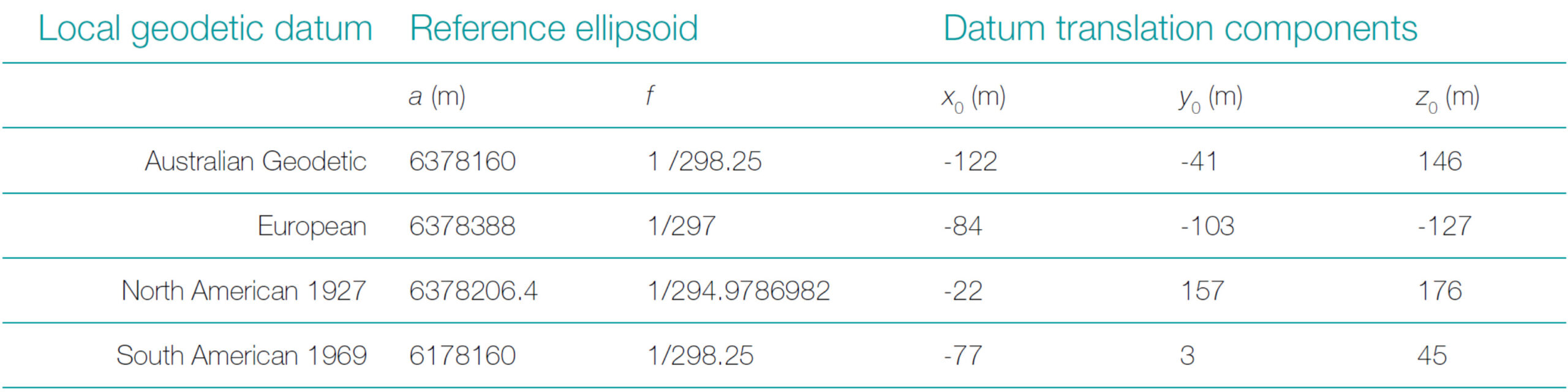
Local geodetic datums, on the other hand, were established long before the dawn of the satellite age. Lacking satellites to locate the geocentre, the stars were used. In the earliest and crudest method, arcs on the terrain were accurately surveyed to find their lengths, and precise astronomic observations were made to find the angles the arcs subtended at the geocentre. The size (semi-major axis a) and shape (semi-minor axis b, or flattening f = (a – b) / a) of a reference ellipsoid could then be computed by comparing the linear and angular lengths of two or more meridian arcs at different latitudes. A reference ellipsoid was chosen because it is the simplest figure which reasonably approximates the shape of the mean sea level surface (which we call the geoid). Having chosen an ellipsoid, it was positioned relative to the earth by specifying the geodetic coordinates (latitude Φ, longitude ʎ, and height h) of a single terrain point, and an initial azimuth to a second terrain point. It was then assumed that the centre of the ellipsoid coincided with the geocentre, whereas in fact the difference was usually several hundred metres. More sophisticated techniques of choosing the ellipsoid size and shape, and positioning it relative lo the earth, have been developed; but the primary limitation (lacking satellites) is that only data from interconnected geodetic networks, that is from a single continent, can be used for each such determination. As a consequence, each continent, and in some cases each country, presently has its own local geodetic datum, reference ellipsoid and implied geocentre location. Table 1 lists the ellipsoid sizes and shapes used with several local geodetic datums, together with the coordinates of the ellipsoid centres expressed in a particular geocentric (satellite) coordinate system called WGS72 (Seppelin, 1974). These datum translation components, as they are called, are Cartesian coordinates in a right handed coordinate system whose Z-axis passes through the north pole and X-axis passes through the intersection of the equator and the Greenwich meridian. (The actual definition of this coordinate system uses more precise language).
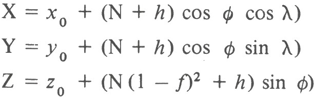
Given the local geodetic coordinates of a terrain point, and values for a, f, x0 , y0 , z0 such as from Table 1, the geocentric Cartesian coordinates of the terrain point can he computed from:
 |
(4) |
where the prime vertical radius of curvature is
| (5) |
Unfortunately, given XYZ it is not so easy to invert Eq. (4) to obtain Φʎh. However there are three ways of doing this; the direct method (Paul, 1973); the differential method (Heiskanen & Moritz, 1967); and the iterative method, which we shall now describe.
9.1 Iterative method
Given X, Y, Z, x , y , z , a and f, we first compute, in order:
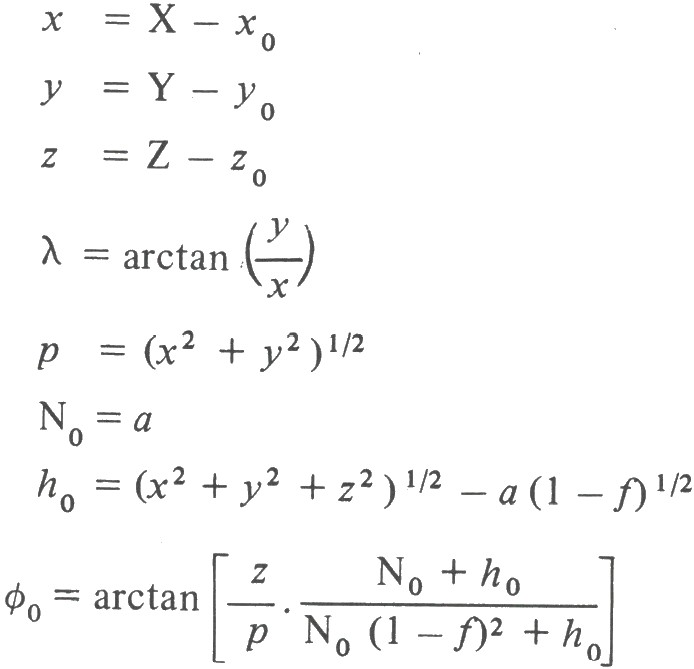 |
Then for the iterations i = 1, 2, 3… we compute, in order:
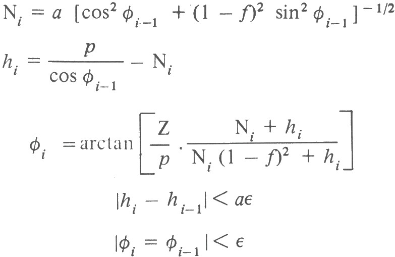 |
(6) |
for some appropriately chosen value of ε (for example ε = 10-7 radians for convergence to one metre or less).
Returning to the problem at hand, we obtain a Navsat position in a geocentric coordinate system (that is x0 = y0 = z0 = 0), but we are interested in trying our Navsat coordinates to the geodetic coordinate system of the closest country or continent. The solution is to first convert Navsat Φʎh to geocentric XYZ using Eq. 4 with x0 = y0 = z0 = 0, and whatever ellipsoid dimensions a and f have been built in to the Navsat computer program used; and then convert the geocentric XYZ thus obtained into geodetic Φʎh iteratively using Eq. 6 with the values for x0 , y0, z0, a, f given for the local geodetic datum.
Note that in both Eq. 4 and 6 the third geodetic coordinate h is the height of the terrain point above the reference ellipsoid, not the height above sea level. Therefore we need to know the height of mean sea level (the geoid) above the ellipsoid used for Navsat computations, so that we can obtain the correct value of h to use in Eq. 4. Maps of geoid heights above the Navsat reference ellipsoid are usually supplied with computer software. One can be found in Moffett (1973).
10 Applications
10.1 A bias-free control for integrated offshore positioning
The great power of Navsat for precise surveying offshore lies in the fact that the position errors, though sizeable, are generally random from one pass to the next. For instance, the effect on the fix of an error in measuring ship’s velocity is equal and opposite for north-going and south going satellites. In contrast, most other electronic positioning methods have high short-term repeatability but suffer from large offsets, or accumulate error with time. The two types complement each other neatly. Good repeatability produces accurate course and speed measurement for computing the satellite fix, and bridges between a number of passes to mean out random Navsat errors. In return, Navsat provides a bias-free control network. Fig. 8 illustrates this symbiosis.
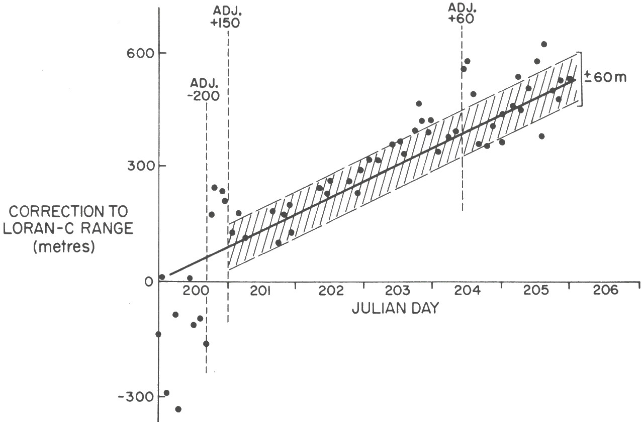
a continuous check on the accumulated clock drift correction. Points represent the difference between
range to the transmitter by Loran-C, and range computed from the Navsat fix.
10.2 Navsat combined with rho-rho Loran-C
In the last decade, portable atomic frequency standards have been developed that are capable of keeping time (which is simply a matter of counting cycles at a known frequency) with an accuracy of a few parts in 1013. If two such clocks had been rated against each other and then sealed in Tutankhamen’s tomb in 1352 B.C., they would have differed by about 1/100 s when re-discovered in the last century.
Precise timing can be used with any radio aid to measure ranges, and hence position the ship. One atomic clock controls the transmitter, while a second operates the receiver, feeding to it a replica of the transmitted signal, at the time it is actually transmitted. The interval between the replica and the arrival of the real signal from the transmitter is the radio wave travel time; given accurate knowledge of propagation this can be converted to range.
The first stage in this so-called “rho-rho” mode of operation is to synchronise the two atomic clocks. It is not necessary to take the receiver physically to the transmitter to do this; entering a known signal travel time is equivalent. To determine travel time, both the distance to the transmitter and the propagation velocity must he known, and since the propagation velocity can only be predicted accurately over water, a good fix at sea is preferred for initial synchronisation. In practice, we use the mean of several days of “good” satellite passes to synchronise to ± 0.1 µs, or ± 30 m (1σ) (Grant, 1973).
Thereafter, continuous comparison with satellite navigation keeps control over the other small systematic errors that can creep into rho-rho positioning. An error of about 5 parts in 1013 is likely in rating the receiver clock alongside the dock before sailing (which is done simply by recording how the range changes with time over at least 24 hours); this introduces range error at the rate of ± 0.05 µs, (± 15 m) per day, and the accumulation will be detected by Navsat after four or five days. Overland errors, station position errors, etc., are also eliminated by a long series of comparisons with Nanat. In fact, one approach to this combination looks on Loran-C purely as a relative motion sensor to track the ship in between satellite passes (Hatch, 1974).
10.3 Navsat and Doppler Sonar
The return echo from an oblique sonar transmission aimed at the seabed ahead of the ship will be Doppler shifted in proportion to the ship’s speed. Matching this with a second transmission aimed astern eliminates errors due to ship’s trim. If another pair of port/starboard transmissions are added, and the whole integrated with a good gyro compass, the resulting system gives very sensitive relative navigation, so long as water depth is less than about 200 m and sea conditions are moderate. Our limited experience of calibrating Doppler Sonar in a harbour against horizontal sextant angle fixes showed an accuracy of better than 0.5 % of distance run.
At sea, Navsat is used to calibrate fixed errors in the gyro, and scale errors in the Doppler measurement, and also to provide the framework of control positions on which to hang the dead reckoning. The measurement of ship’s track during the pass is smooth, and the response to alterations in course and speed immediate. This makes Doppler sonar better at providing velocity for the calculation of satellite fixes than most radio navaids, which are relatively “noisy”.
When using Doppler sonar, the ship’s track can justifiably be broken into 20 s intervals for computing the Navsat fix. This refinement is probably not obtainable from very-long-range radio positioning methods, such as Loran-C, because they are too noisy to define a short track segment. Stansell (1973) estimates that the use of 20 s Doppler intervals improves Navsat accuracy from ± 100 m to ± 60 m.
10.4 Cycle identification by Navsat
All phase comparison and cycle matching radio aids resolve only the fraction of a cycle; they rely on auxiliary measurements to determine the whole number of cycles in the reading. These “coarse” measurements tend to become ambiguous just when they are needed most: at long range or under adverse radio conditions. The traditional solution of the surveyor has been to lay buoys as “lane markers”. In order to give the resolution required, these must be laid in shallow water, to restrict their radius of swing, and they are often lost in storms or to trawlers. Many valuable survey hours have been lost in the past steaming to a buoy to re-set lost lanes.
The Navsat accuracy of ± 120 m from about two thirds of all good passes means that Decca lane identification (± 180 m required) is usually acquired on the first pass, and rho-rho Loran-C cycle identification (± 1500 m required) is assured. Even for medium frequency radio aids with a half lanewidth of around 40 m, there is about 50 % probability of being within ± 1 lane; this means that useful work can often be done on the run in to the marker buoy, even if positions must be adjusted by one lane afterwards.
10.5 Calibrating radio aids
Long range survey positioning systems are usually calibrated within line of sight of the transmitter (when safe navigation permits) but are used at much greater ranges. The Surveyor assumes that short range calibration, plus knowledge of the radio wave propagation velocity, is valid in the distant survey area. Now these calibrations and velocity assumptions can he checked by making a large number of Navsat comparisons during the survey.
Overland signal path, with its unpredictable propagation velocity, may sometimes be unavoidable. Navsat can be used to give a first approximation to the overland phase lag corrections, although the accuracy will be lower than for an all-over-water path because the corrections will usually vary rapidly with location as the proportion of land path changes. If a good model for the phase lag corrections is available, Navsat will give spot checks on the model to validate or adjust the predictions.
“Main Chain” aids to commercial navigation can also be calibrated very economically for latticing small scale charts. We recently ran a Decca and Loran-C test calibration in the Gulf of Maine; the agreement between calibrations and comparisons with previous fixed-error corrections indicated a calibration accuracy of ± 300 m (2σ). We had no need to set up a local high accuracy radio system to do the calibration, nor did we have to depend on seeing the land for visual fixes.
10.6 Shore control and geodesy
Navsat was designed for navigating submarines. It is a striking testimony to the powerful technique of meaning out random errors by accumulating a large number of satellite passes, that one of its major applications has been in geodesy. The results of five days’ observations at one point will give a position consistent with other Navsat positions within a very few metres; “consistent” because it will differ from positions on the local survey network by the datum shift. At this level of accuracy, small systematic errors, such as residual refraction errors, become noticeable, and precision is further improved by the “translocation” technique of measuring interstation distances by making measurements on the same satellite simultaneously at two or more stations. Doppler satellite distances observed this way agree with geodetic triangulation within 1–3 metres over both short lines (less than 200 km) and long lines (1000 km). (See for example Anderle, 1974; Khakiwsky, 1973; and Kouba, 1974).
Fixed site surveys by Navsat require none of the precise and laborious observations of high order control surveys. All one needs is a portable receiver, an attendant to change tapes, and a good 3-D computer program to process the results afterwards.
Navsat is also used for fixing the position of long range navaid transmitters, and to provide geographic position for shore control for hydrographic surveys (Finnegan, 1971). It has recently become the standard method of positioning offshore oil drilling rigs in Canadian waters, satisfying both legal and operational requirements, with an accuracy of ± 15 m (Hittel, 1971).
Acknowledgements
Satnav was, to our knowledge, first used for Decca Jane identification by Shell (Canada) Ltd., in 1970. We thank Mobil (Canada) Ltd. and Dabbs Control Surveys Ltd. for the opportunity to test Doppler Sonar.
References
Anderle, R. J. (1974). Transformation of Terrestrial Survey Data to Doppler Satellite Datum. Journal of Geophysical Research, Vol. 79, No. 35.
Brunavs, P. and Wells, D. E. (1971). Accurate Phase Lag Measurements over Sea Water Using Lambda Decca, Report AOL 1971-2. Bedford Institute of Oceanography, Dartmouth, Canada.
Bryant, Eaton, and Grant (1974). Rho-rho Loran-C for Precise Long Range Positioning Inland and at Sea. Proceedings of the 14th International Congress of Surveyors, Washington.
Finnegan, E. W. (1971). Geodetic Applications of a portable Doppler Satellite Receiver. Paper submitted at the 13th International Congress of Surveyors, Wiesbaden.
Grant, S. T. (1973). Rho-rho Loran-C combined with Satellite Navigation for Offshore Surveys. Int. Hydrog. Review, Vol. L (2), pp. 35–54.
Guier, W. H. (1965). Satellite Geodesy. APL Technical Digest, 4, No. 3, 2–12.
Hatch, R. R. and Winterhalter, J. J. (1974). Differential Loran-C in Integrated Marine Navigation Systems. International Symposium on Applications of Marine Geodesy, Battelle Memorial Institute, Columbus, Ohio, U.S.A.
Heiskanen, W. A. and Moritz, H. (1967). Physical Geodesy. W. H. Freeman & Co., San Francisco.
Hittel, A. and Kouba, J. (1971). Accuracy Tests of Doppler Satellite Positioning in Orbital, Translocation and Simultaneous Modes. Given at the 13th International Congress of Surveyors, Wiesbaden.
Hopfield, H. S. and Utterback, H. K. (1973). Tropospheric effect on electromagnetic range measurement at oblique angles. Transactions of the American Geophysical Union, 54, 232 (Abstract). Johler, J. R., Kellar, W. J., and Walters, L. C. (1956). Phase of the Low Frequency Ground Wave. U.S. National Bureau of Standards Circular 573.
Krakiwsky, E. J., Wells, D. E., and Thomson, D. B. (1973). Geodetic Control from Doppler Satellite Observations for Lines under 200 km. The Canadian Surveyor, Vol. 27 (2).
Kouba, J., Peterson, A. E., and Boal, J. D. (1974). Recent Canadian Experience in Doppler Satellite Surveying. 14th International Congress of Surveyors, Washington, D.C.
Moffett, J. B. (1971). Program Requirements for Two-minute Doppler Satellite Navigation Solution. Johns Hopkins University. Distributed by N.T.I.S., 5285 Port Royal Road, Springfield Va. 22151, U.S.A.
Paul, M. K. (1973). A note on the computation of geodetic coordinates from geodetic (Cartesian) coordinates. Bulletin Geodesique, No. 108.
Seppelin, T. D. (1972). The (U.S.) Department of Defense World Geodetic System 1972. International Symposium on Problems Related to the Redefinition of North American Geodetic Networks, University of New Brunswick, Fredericton, Canada.
Stansell, T. A. Jr. (1968). The Navy Navigation Satellite System: Description and Status. Navigation (Journal of the U.S. Institute of Nav.), Vol. 15 (3). Reprinted in lnt. Hydrog. Review, Vol. XLVII (1), pp. 51–70.
Stansell, T. A. Jr. (1973). Accuracy of Geophysical Offshore Navigation Systems. Offshore Technology Conference, OTC 1789.