


Abstract
1 Introduction
The seabed near the coast is constantly changing as a result of natural processes and human activities. On the one hand, erosion by waves, currents and tides leads to the removal of material. On the other hand, the deposition of sediments can cause the seabed to rise. Human activities such as the extraction of sand or gravel for construction purposes, the building of coastal engineering structures and the dredging of shipping channels can also lead to changes in the seabed and affect erosion or sedimentation processes (De Groot, 1986; Kubicki et al., 2007; Mielck et al., 2018; Hendriks, 2020; Ratrick et al. 1992; Bian et al. 2022).
Permanent changes of submarine topography require continuous monitoring of the seabed to provide early response to changes, take protective measures, minimize environmental impacts, and ensure the safety of coastal communities and infrastructure. Accurate information on submarine topography is essential for safe ship navigation, adequate infrastructure planning, appropriate coastal protection and a wide range of environmental applications such as eco-hydraulics, habitat modelling, and investigation of littoral vegetation (Korhonen, 2014; Mandlburger, 2021; Christiansen, 2021; Jonas, 2023; Hecht, 2023).
The topography of the seabed can be mapped using a variety of methods that differ in resolution, area coverage, achievable water depth and accuracy. For the global acquisition of low-resolution deep water bathymetry data, satellite altimetry and satellite gravimetry are used. Both methods do not directly measure water depth. Satellite altimeters determine the height of the water surface, which, among many other effects, depends on the gravity of the submarine topography. The water depth can then be estimated using gravity models (Sandwell et al., 2014; Wölfl et al., 2019). In satellite gravimetry, the topography of the seabed is derived indirectly from gravity measurements (Smith & Sandwell, 1994; Fan et al., 2020). In smaller study areas, airborne gravimetry (An, 2019) can also be used.
The global acquisition of low-resolution shallow water bathymetry data can be achieved with satellite altimetry and satellite-derived bathymetry (SDB). In shallow waters the advanced high-resolution topographic laser altimeter system (ATLAS) of ICESat-2 is able to detect both water surface and seabed signal photons from which the submarine topography is derived (Parrish et al., 2019; Guo et al., 2022). In areas of clear water, SDB can be used to derive information about submarine topography from multispectral satellite imagery (Hartmann et al., 2022; Laporte et al., 2023). The water depth can be determined by analyzing the attenuation of the radiation at different wavelengths (Pe’eri et al., 2014; IHO-IOC, 2018; Wölfl et al., 2019).
High-resolution bathymetry data is usually acquired using hydroacoustic methods, which are suitable for both deep water and shallow water bathymetry. The water depth can be determined using echo sounding. Single Beam Echo Sounders (SBES) map the submarine topography along a narrow survey line strip, while Multi Beam Echo Sounders (MBES) record a wide swath of the seabed (Pandian et al., 2009). The spatial resolution of these systems depends on the beam aperture, water depth and incidence angle of the beam’s boresight angle to the local seabed (Lurton, 2002). Very high spatial resolution can be achieved in shallow water. However, collecting bathymetric data with shipborne systems in shallow water is substantially more time-consuming than collecting deep-water data. Time windows limited by tidal effects and long transits of survey launch vessels further reduce the efficiency, so that echo sounding in shallow water areas reaches its limits.
Airborne LiDAR bathymetry (ALB) is an alternative technique that enables the time-efficient and area-wide survey of submarine topography in coastal shallow water areas with a high point density (Ellmer et al., 2014; Mandlburger, 2020) and in compliance with the Total Vertical Uncertainty (TVU) requirement of IHO S-44 Special Order (IHO, 2020; Mandlburger, 2022). ALB systems, mounted on a crewed or uncrewed airborne platform, emit short green-wavelength laser pulses and record their return from the water surface, water column and seabed (Fig. 1a). During the transition of the laser pulse from air to water, changes in the propagation direction and propagation speed of the laser pulse must be considered (refraction correction). The complete shape of the backscattered signal is digitized with high temporal resolution. The result is a so-called full-waveform (FWF) with a pronounced signal maximum at the water surface, an exponential signal decay in the water column and a second, significantly weaker maximum at the water bottom (Guenther et al., 2000; Fig. 1b). The difference in time between water surface return and seabed return is used to determine the water depth. However, green laser light cannot accurately determine the actual water surface (Guenther, 1985). Due to its penetration properties, the water surface is systematically underestimated by 10–25 cm (Mandlburger et al., 2013) resulting in a systematic error at the seabed. For this reason, many ALB systems also use a near-infrared laser that simultaneously scans the water surface. Due to its significantly lower penetration depth (Guenther et al., 2000; Mandlburger, 2022), it can provide accurate information on the actual water surface height.
(b) Elements of a full-waveform.
State-of-the art processing methods perform online waveform processing (OWP; Pfennigbauer et al., 2009; Pfennigbauer & Ullrich. 2010), where the local maxima of water surface and bottom are derived automatically via peak detection methods. If the seabed echo is weak due to high turbidity or greater water depth, the OWP may fail. Full-waveform stacking methods, which can detect even weak bottom echoes by combining neighboring signals, may prove beneficial in these circumstances. Note that the term “online waveform processing (OWP)” is used by the sensor manufacturer RIEGL to refer to real-time (i.e., during data acquisition) waveform processing applied in the firmware or manufacturer software.
The article is structured in six sections, starting with the introduction. Section 2 summarizes recent developments on full-waveform stacking and presents the contribution of this article to the field of research. Section 3 briefly describes the functioning of the two full-waveform stacking techniques and discusses the method for considering near-infrared water surface information. Section 4 provides a description of the study area and the data available for both processing and validating the results. A visual and quantitative evaluation of the processing results obtained is presented in Section 5. The paper concludes with a brief summary in Section 6.
2 State of the art and research contribution
Recent developments in novel processing techniques, such as signal-based and volumetric full-waveform stacking (sigFWFS and volFWFS), aim to increase the analyzable water depth by jointly analyzing closely adjacent measurements thus providing additional local information about the seabed. By combining the measurement signals in a non-linear approach, the signal-to-noise ratio is improved while avoiding smoothing effects. As a result, even weak seabed signals that are not detected by standard processing methods can be reliably detected.
The goal of sigFWFS and volFWFS is to improve the signal-to-noise ratio of the full-waveforms und make weak bottom echoes detectable. However, they differ in terms of neighborhood definition and consideration of underwater laser pulse propagation. In the sigFWFS processing (Mader et al., 2019, 2021), individual full-waveforms with a neighborhood directly at the water surface are combined into a pseudo full-waveform (stacked full-waveform) by summing the amplitude signals (similar to Stilla et al., 2007; Plenkers et al., 2013; Roncat & Mandlburger, 2016). The propagation of the laser beams in the water column, which can vary significantly due to different incidence angles and refraction at the water surface, is not taken into account. The volFWFS in Mader et al. (2023) accounts for the path of the laser beam through the entire water column by transferring the full-waveforms information into a voxel space (similar to Pan et al., 2016).
Both full-waveform stacking approaches were applied to ALB data of an inland waterway with high turbidity and compared to hydroacoustic measurements. The results show a significant increase in the analyzable water depth of up to + 27 % (sigFWFS) and + 33 % (volFWFS), which allowed a significantly larger area of the riverbed to be mapped. The increase in coverage was respectively approximately + 104 % for the sigFWFS and approximately + 113 % for the volFWFS. Extensive analysis indicated a good representation of the riverbed.
The potential of sigFWFS and volFWFS has already been demonstrated on an inland waterway in the publications mentioned above. For inland waters, the water surface can be assumed to be a horizontal surface that remains static between multiple flight strips. Small waves or ripples can be neglected. However, these assumptions are often no longer valid for marine waters with larger waves and time-varying sea states and must be assessed accordingly. This article is the first to examine the application of the full-waveform stacking approaches to offshore environments. Currently, full-waveform stacking techniques are limited to the processing of the green laser measurements, known to be affected by an underestimation of the water surface height. In this paper, a modified full-waveform stacking approach is presented that allows the use of near-infrared water surface information. This paper proposes to investigate whether the application of sigFWFS and volFWFS to coastal airborne LiDAR bathymetry data can increase the analyzable water depth and consequently improve seabed representation.
3 Methods
In this section, the methods and processing procedures are presented, starting with the estimation of the refractive index (Section 3.1). This is followed by the classification of green laser measurements into water column points (relevant for the full-waveform stacking processing) and seabed points (Section 3.2). After classification, the procedure for water surface correction based on near-infrared and green laser measurements is shown in Section 3.3. For the water surface correction, it is important to note that the green and near-infrared lasers scan simultaneously, but not coaxially, i.e., the water surface is scanned at different locations at the same time, resulting in the detection of two different wave patterns.
The full-waveform stacking approaches are presented in Sections 3.4 (sigFWFS) and 3.5 (volFWFS). In both full-waveform stacking approaches, a neighborhood definition (Sections 3.4.1 and 3.5.1) is performed first, i.e., the measurement area is divided into processing units and the measurement data is assigned to them with respect to their position. For each processing unit, pseudo full-waveforms are generated and analyzed. The result is an initial water depth for each processing unit, serving the basis for the definition of so-called search corridors (Sections 3.4.2 and 3.5.2). The search corridors are then applied to the individual measurements (individual full-waveforms) in order to extract water bottom points (Section 3.6). The application of the search corridors to the individual full-waveforms is intended to avoid a reduction of the measurement resolution. In Fig. 2, an overview of the presented methods, their results and the corresponding section in the method-section are given.
Section 3.7 briefly discusses the evaluation methods for comparing between re-processed seabed points and the hydroacoustic measurements. At the end of this section, the validation methods of the sigFWFS and volFWFS processing of bathymetric data are shown.
3.1 Estimating of the refraction index
During the transition of the laser pulse from air to water, the propagation velocity (both magnitude and direction) changes. Therefore, a refraction correction based on Snell’s law must be applied. For a correct adjustment of the magnitude and direction of the laser pulse in the water column, a correct refractive index of water nw has to be used. Often nW is set to 1.33 or 1.333 and consequently cW is approximately 2.25·108 m/s. However, nW and thus cW depend on the water properties (salinity, temperature and pressure) and the wavelength of the light.
The refractive index for the North Sea was estimated according to the rule of thumb (Eq. 1) of Höhle (1971), where only the numerical values without units are inserted.
|
with
λ … wavelength of the ALB system in [nm]
T … temperature of the water in [°C]
DWD … water depth in [m]
S … salinity in ‰
For the full-waveform stacking processing the salinity was set to 35 ‰ and the temperature was set to 18 °C. These values are consistent with measured values from the six CTD profiles collected during the hydroacoustic survey of the study area (Section 4). Using λ = 532 nm and DWD = 3.0m, the nW is 1.3424 and consequently the cw is 2.2332·108 m/s.
3.2 Classification of the green laser measurements
The evaluation of the green laser measurements using standard processing methods such as OWP often results in a point cloud with some false points above the water surface acquired by the near-infrared laser (nirWS), numerous points in the water column a few centimeters below the nirWS, and a number of points at the seabed. The goal of the classificationis to extract all points of the green laser that have interacted with the water column. Only points derived from the first significant system response/peak in the full-waveform are considered (green first echo point). For this purpose, a simple height-based point classification based on the nirWS-height is performed. All points below the nirWS that are not bottom points are classified as water column points and are included in the full-waveform processing. The bottom points are clearly different in height from the other points and can be easily distinguished from them. For this pilot study, the classification method involved interactively setting height thresholds. Commercial classification software/modules or artificial intelligence (AI) approaches are also viable options, for instances Letard et al. (2021). Fig. 3 shows an example of a point cloud before and after classification.
3.3 Water surface correction
The classified water column points described in Section 3.2 and their corresponding full-waveforms are the basis for the subsequent sigFWFS and volFWFS processing. However, due to the penetration properties of the green laser, these points are several centimeters deeper than the actual water surface. The aim of the water surface correction is to correct this underestimation using the near-infrared laser data. Due to the simultaneous but not coaxial scanning of the water surface by the green and near-infrared lasers, the following important aspects must be considered when correcting the water surface:
- The correction of the height component of the water surface is performed using the measurements of the near-infrared laser pulses.
- The surface shape (waves) is derived from the measurements of the green laser pulses.
The water surface correction is based on the following assumptions:
- The green first echo point is derived from the first significant system response (= peak or echo) in the full-waveform.
- The green first echo points were not subjected to refraction correction during preprocessing.
- Noise effects are random and normally distributed.
- The shape of the water surface can be derived from the green first echo points by modeling.
For the realization of the correction, the following steps were executed:
- Determination of a water surface model based on the near-infrared first echo points; this corresponds to the best approximation of the actual water surface height (Fig. 4a).
- Determination of the height differences di between nirWS and green first echo points Pgreen_original (Fig. 4a).
- Averaging of all height differences (dmean) and shifting the Pgreen_original points to the height of the nirWSmodel → Pgreen_corr,ws (Fig. 4b; yellow arrow).
- Calculation of the water surface model based on the Pgreen_corr,ws points; this water surface model is characterized by the wave pattern of the green laser pulse measurements and the height of the nirWS (Fig. 4b).
- Calculation of the corrected green first echo points in the water column (Pgreen_corr,ws) considering refraction correction and velocity reduction on corrected green water surface model (Fig. 5).
3.4 Non-linear signal-based full-waveform stacking – sigFWFS
In the following, the three processing steps of the sigFWFS are briefly introduced, starting with the neighborhood definition to assign the measurement data into processing units (Section 3.4.1). The core processing step of the sigFWFS involves the stacking of the measurement data into a pseudo full-waveform (= stacked full-waveform; Section 3.4.2) and the detection of the water bottom echo in the pseudo full-waveform. The final processing step, detection and extraction of seabed points, is very similar as in volFWFS and is shown in Section 3.6.
3.4.1 Neighborhood definition
In sigFWFS, the neighborhood definition is realized by a regular 2D grid close to the water surface (green first echo points), whose grid cells represent the processing units (Fig. 6). All data whose XY coordinates of the first echo point fall within a processing unit are processed together. The size of the grid cell or processing unit may vary depending on the spatial resolution and distribution of the measurement data, as well as on the seabed local topography, i.e. bottom slope. This simple form of neighborhood definition is limited to the water surface. However, as the laser pulses hit a dynamic water surface at different angles, their direction of propagation in the water column differ. Therefore, a neighborhood at the water surface does not necessarily lead to a neighborhood in the water column and at the seabed.
3.4.2 Full-waveform stacking and definition of the search corridor
In Mader et al. (2019, 2021), the actual analysis of water depth begins with the generation of the pseudo full-waveforms (stacked full-waveform) after the full-waveforms have been assigned to the processing units. This involves aligning all full-waveforms of a processing unit to each other and summing up their amplitudes (Fig. 7a). The analysis of the stacked full-waveform provides the necessary information regarding approximate water depth (= number of samples between alignment height and seabed echo) and information on the slope of the seabed (= peak width of bottom echo) to detect weak bottom echoes in the individual full-waveforms. Additional filtering and control methods (e.g., use of reliably detected seabed echoes as control values, mutual control of water depths of processing units) ensure high reliability of water depth information from stacked full-waveforms. Finally, a search corridor can be determined for all individual full-waveforms of the same processing unit. The location of the search corridor is determined by the approximate water depth (NoSsb). The width of the search corridor is derived from the peak width to account for local slope differences within the processing unit (Fig. 8).
For the application to marine waters, the procedure was refined with the goal of eliminating the effects of wavy and unsteady water surfaces on the sigFWFS. Firstly, all individual full-waveforms of a processing unit are no longer aligned at the peak of the water surface, but at a fixed height (alignment height; Fig. 7a). This can be achieved by utilizing the geometric path of the green laser beam, the position of the green water surface echo (= Pgreen_corr,wc) and the known time duration between two samples (sample time interval). Secondly, the seabed peak is no longer identified as the most significant peak after the water surface peak. In the resulting stacked full-waveform, the seabed peak is detected by searching for the most significant echo in a defined search area between the lowest first echos (of the full-waveforms) and the end of the full-waveform (Fig. 7b).
3.5 Non-linear volumetric full-waveform stacking – volFWFS
This section briefly introduces the volFWFS, which differs from the sigFWFS (Section 3.4.1) in the definition of the neighborhood and the generation of the pseudo full-waveform (= ortho full-waveform). However, the most important improvement is the geometric consideration of the laser pulse path, which guarantees the geometric neighborhood of the measured values throughout the water column.
3.5.1 Neighborhood definition
In volFWFS, the assignment of closely neighboring ALB measurements is realized using a local voxel space representation (Fig. 9). In contrast to sigFWFS, the neighborhood definition of full-waveforms is no longer limited to the water surface, but comprises the entire water column in a Cartesian system. The transfer of full-waveform data into the voxel space is performed by assigning each full-waveform amplitude point to the corresponding voxel with respect to the spatial position (Fig. 10a).

3.5.2 Full-waveform stacking and definition of the search corridor
Vertical voxel columns are used as processing units, which are the basis for ortho full-waveform generation (Fig. 9). For this purpose, an ortho full-waveform is generated from the averaged amplitude values of the voxel column (Fig. 10b). In the ortho full-waveform, the bottom echo is detected similarly as in the sigFWFS (including the filter algorithm) and used for determination of an initial seabed model from which water depths can be derived for further processing (Fig. 11). The seabed model consists of a regular grid of points (distance = horizontal voxel size). The height information between the points can be determined by interpolation methods.
The sampling distance (NoSsb) between the green first echo point (Pgreen_corr,wc) and the initial seabed point (Psbm) is derived from the seabed model and the known propagation direction of the green laser pulse in the water body (Fig. 11). Together with the peak width (analogous to sigFWFS), the search corridor can be defined and used to detect the bottom echo in the individual full-waveform.
3.6 Detection and extraction of seabed points
In a final processing step, the search corridor determined in Sections 3.4.2 or 3.5.2 is used to restrict the search area of the seabed echo in the individual full-waveform. For sigFWFS, the search corridor can be transferred directly from the stacked full-waveform to the individual full-waveform (Fig. 8). In the case of volFWFS, the search corridor is derived from the seabed model and the beam path of the individual full-waveform (Fig. 11). This approach greatly reduces the number of possible bottom echoes. The local maximum with the least number of samples to NoSsb is assumed to be the seabed echo (Figs. 8 and 11). If there is no echo within the search corridor, no seabed point will be extracted. Finally, based on the detected seabed echo and the known beam geometry of the laser pulse, the seabed point can be calculated. Therefore, the corrected green first echo point Pgreen_corr,wc is the corresponding point to the first object echo in the full-waveforms (= “water surface echo” in Fig. 1b) and thus also the starting point for the calculation of the seabed points. The approach of applying a search corridor to the individual measured full-waveforms is equivalent to a modified majority voting instead of averaging, thus avoiding low-pass filter effects. This is the reason for using the term non-linear full-waveform stacking. In this way smoothing effects of full-waveform stacking are avoided and the seabed is represented by a larger number of 3D points.
3.7 Evaluation methods
For a proper evaluation of the results, a comparison between the seabed points from full-waveform processing and the hydroacoustic measurements (Section 4.2) is performed in Section 5. The evaluation of the comparison is carried out both visually, by presenting cross sections, and quantitatively, by providing the following statistics:
-
mean height difference
 to detect trends in whether the reprocessed points are too high or too low
- root mean square (RMS) as a standard value for general assessment of accuracy
- standard deviation of the median absolute deviation sMAD (Hampel, 1974; Sachs, 1982) – similar to RMS, but without possible systematic errors
-
inlier rate, which indicates the proportion of points that do not exceed a specified limit (Litman et al., 2015); multiple of
 and the TVU of IHO S-44 Special Order (at a water depth of about 4 m) was used as a metric for the limit
The quantitative evaluation is carried out globally for all points and also as a function of water depth, as Mader et al. (2021, 2023) showed that the values can vary with water depth. The , RMS, sMAD are used for accuracy, and the inlier rate is used for reliability.
4 Study area and dataset
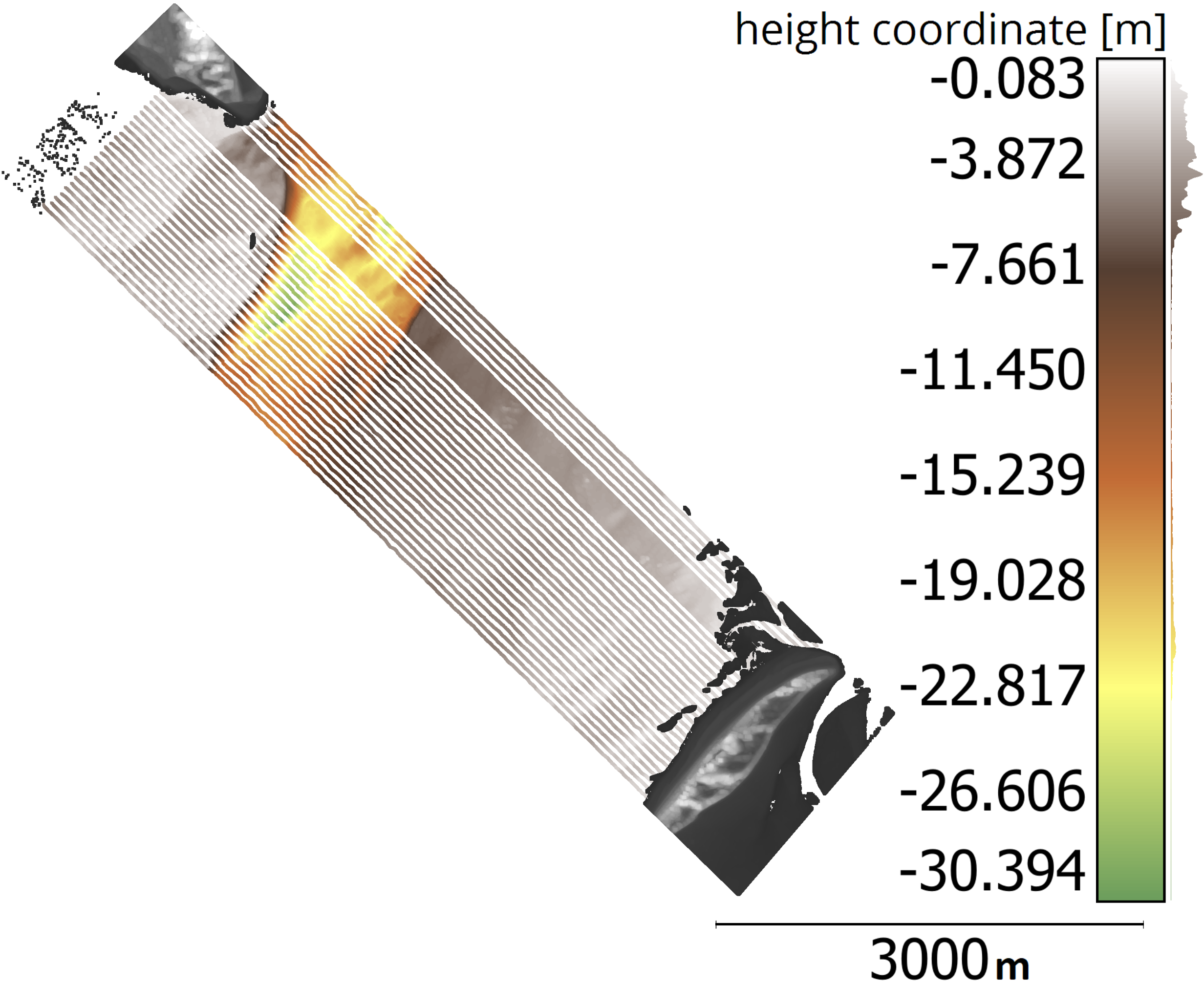
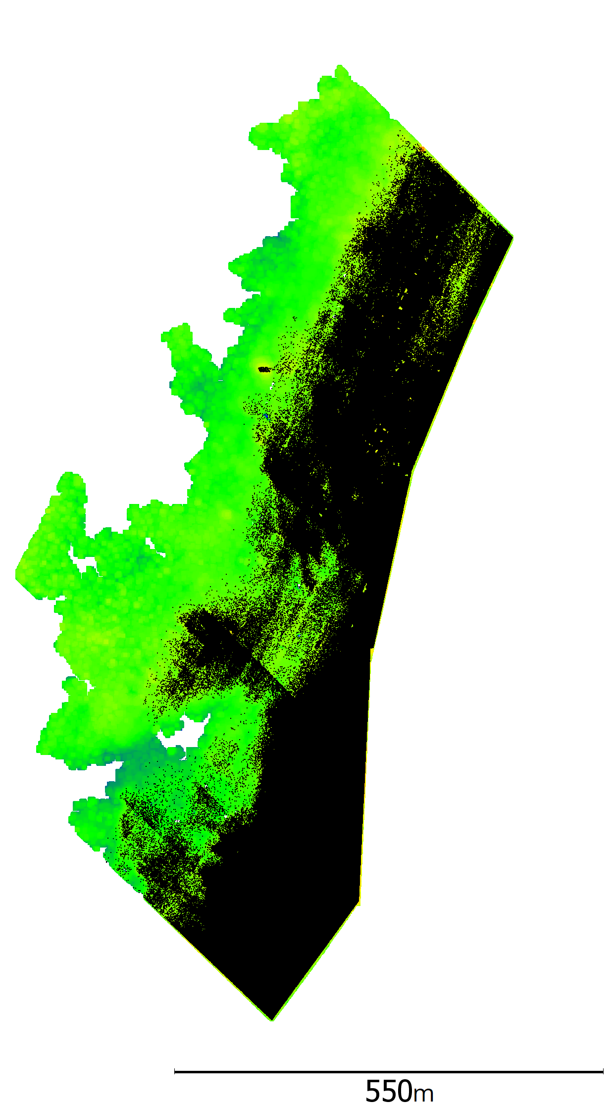
The study area is located in the German Wadden Sea National Park between the islands of Sylt (to the northwest) and Amrum (to the southeast) and has an extent of about 7.5 km × 1.9 km surveyed in twelve overlapping flight strips and two cross strips (Fig. 12). The ALB data were acquired in mid-August 2021 with the ALB system RIEGL VQ-880-G II. The green laser of the RIEGL VQ-880-G II operates at a wavelength of 532 nm, a pulse repetition rate (PRR) of 700 kHz, and a sensor-side beam divergence of 2.0 mrad. It had a beam deflection angle of 20°, resulting in an elliptical footprint of approximately 1.2 m × 1.1 m (major axis × minor axis) on a horizontal surface at an average flight altitude of about 540 m above the water surface. The sample time interval for the recorded full-waveforms was 5.75·10-10 s and corresponds to a 3D distance of 6.42 cm under water (using the cW from section 3.1). A spot check of the point density at the water surface showed a minimum point density of 13 points/m2 to 19 points/m2 depending on the flight strip. The flight strips are processed together resulting in an even higher point density due to the overlap of the strips and the characteristics of the ALB system’s scan pattern (circular scan pattern).
4.1 Study area
For the full-waveform stacking processing of the ALB data, a subarea with a manageable data size and slowly increasing water depth was selected to demonstrate the potential of full-waveform stacking in coastal waters. Fig. 13 shows the location of the 900 m long and between 180 m and 260 m wide subarea within the study area. The measurement data were processed using both sigFWFS and volFWFS. In empirical studies (Mader et al., 2021, 2023) using the RIEGL VQ-880-G ALB system with comparable point density and scan pattern, test areas with different raster cell and voxel sizes were processed and evaluated with respect to the achieved accuracy and reliability as well as the number of extracted points. The results for grid cell sizes from 2.0 m × 2.0 m to 2.5 m × 2.5 m and voxel sizes from 2.0 m × 2.0 m × 0.10 m to 4.0 m × 4.0 m × 0.14 m were very similar, so grid cells of 2.5 m × 2.5 m and voxels of 2.5 m × 2.5 m × 0.1 m were selected for processing the ALB North Sea data.
4.2 Dataset
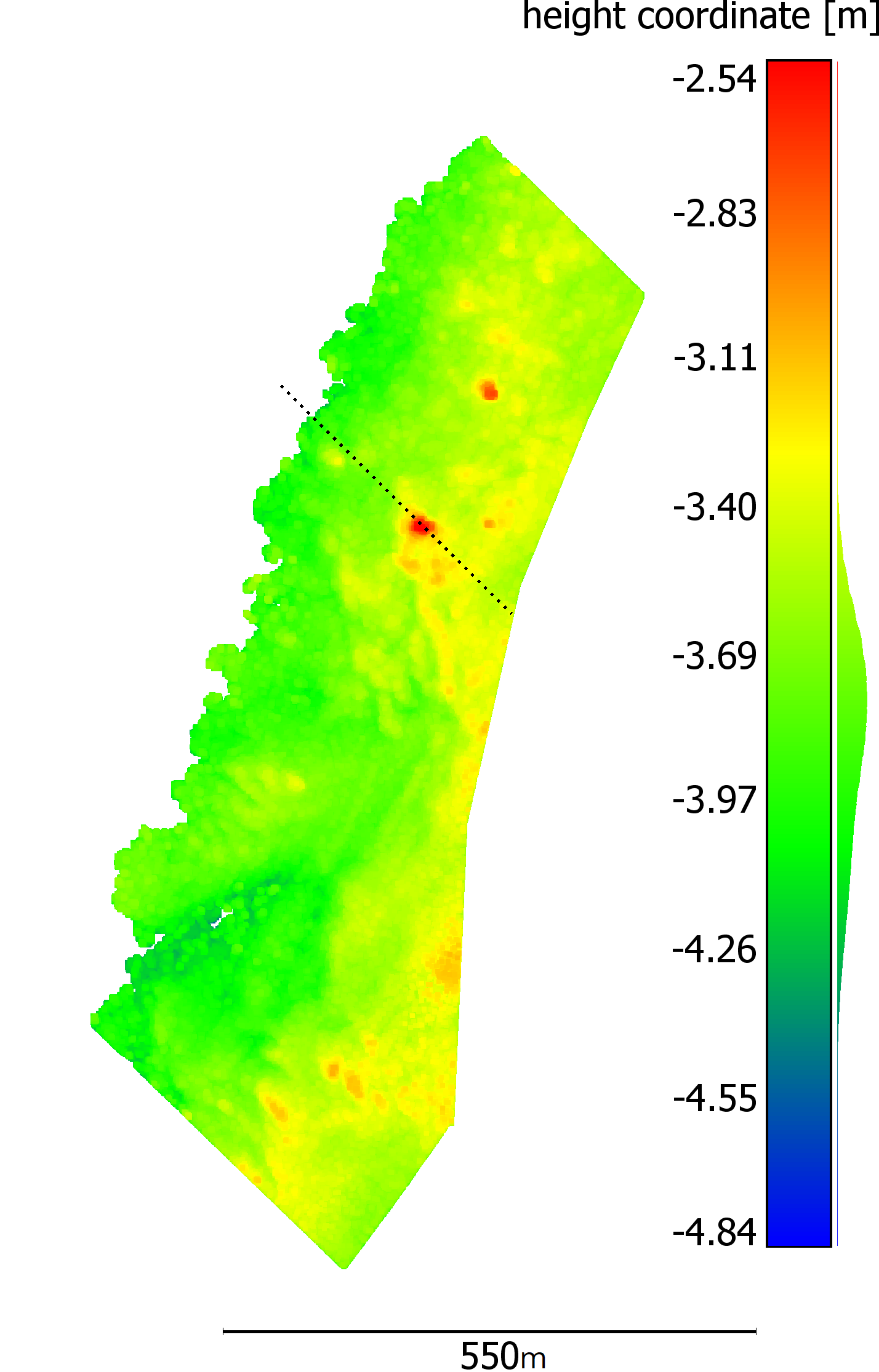
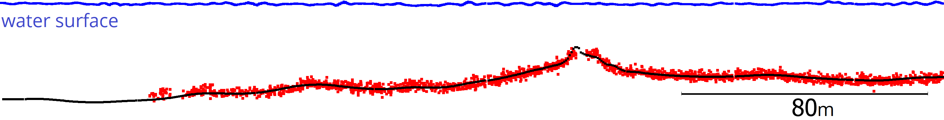
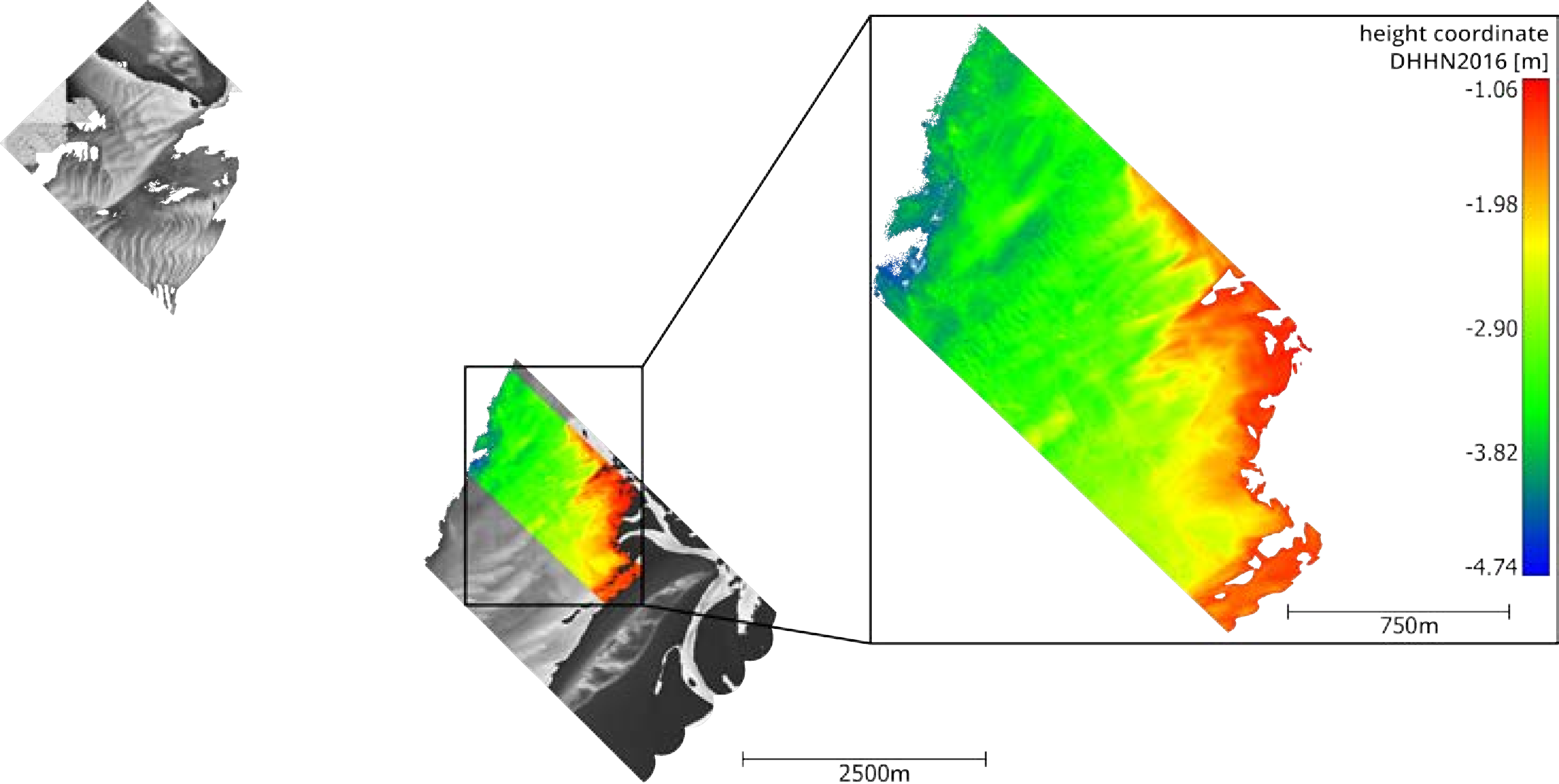
Fig. 14a shows the OWP point cloud resulting from standard processing by an airborne service provider. The classified seabed points are color coded according to their height coordinate in the national height reference frame of Germany (DHHN2016). The land points are colored gray. Although the OWP data already cover a large part of the study area, the method reaches its limits in the middle of the area, resulting in a data gap.
The results of the full-waveform stacking were compared to hydroacoustic measurements (Fig. 14b) collected during two surveys, respectively one and three weeks after the airborne data acquisition. During this time, no storm event in the study area occurred that would have caused major changes in the bottom topography. The hydroacoustic surveys were carried out by two BSH survey launches equipped with Kongsberg Maritime EA440 SBES (38/200 CombiD transducers). Two sound speed profiles per survey day were acquired using a Sea & Sun CTD60 profiler and used for time-of-flight to depth conversion. The maximum mean sound speed difference in a single day was 0.6 m/s. An IXblue Octans Surface attitude and heading reference system was used for heave corrections. A Leica GX1230+ GNSS receiver was used for position determination, augmented by high precision real-time corrections provided by the national satellite positioning service of Germany, SAPOS. The cm-level accuracy achievable allows for Ellipsoidal Referenced Survey (ERS). Depth measurements were further reduced to normal heights using the German Combined Quasigeoid (GCG2016). A series of four control lines, orthogonal to the survey lines, were collected by both survey launches. An a posteriori uncertainty of 17 cm (95 % confidence interval) was calculated from the 64 intersection points between control and survey lines. The survey line spacing was 50 m, with an approximately 200m wide strip surveyed with a 10 m line spacing. Due to the lack of full bathymetric coverage however, only points close to the hydroacoustic measurements are included in the comparison for result evaluation.
5 Results
In this section, the results of the sigFWFS and volFWFS processing are compared with the hydroacoustic measurements. First, a visual comparison is made using a cross section, followed by a quantitative analysis. Finally, the benefit of the full-waveform stacking processing compared to the standard processing methods is shown.
5.1 Visualization of the results
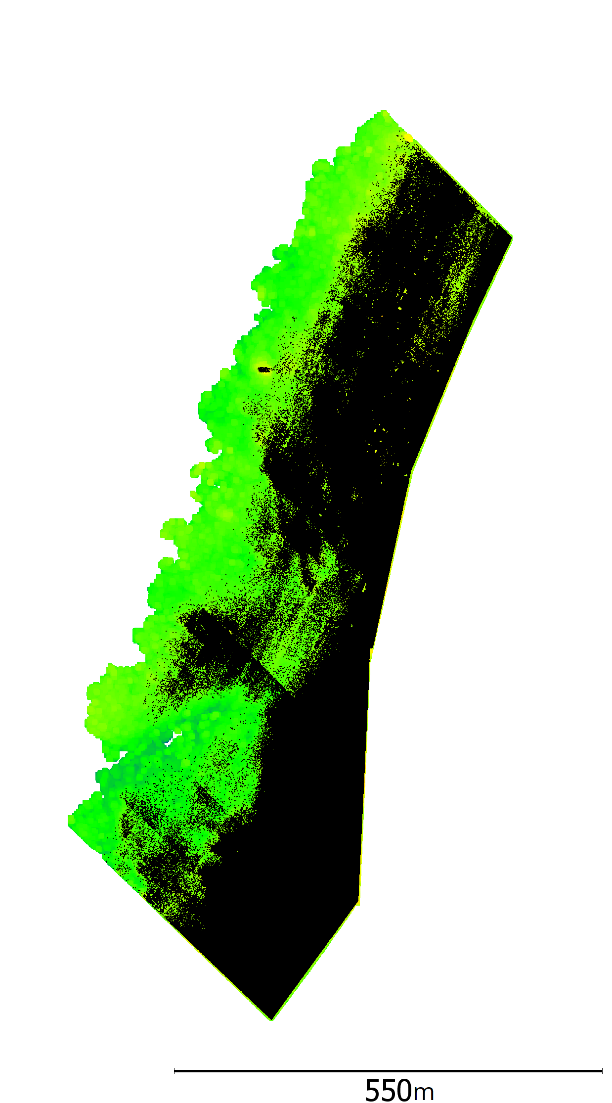
The full-waveform stacking point clouds are shown in Figs. 15a and 15c. Both have the same characteristics of seabed topography (elevations and sinks) as the OWP data in Fig. 13. A comparison of seabed coverage between the newly processed points and the OWP points (Figs. 15b and 15d) shows a significant increase in the number of seabed points for the sigFWFS and the volFWFS.
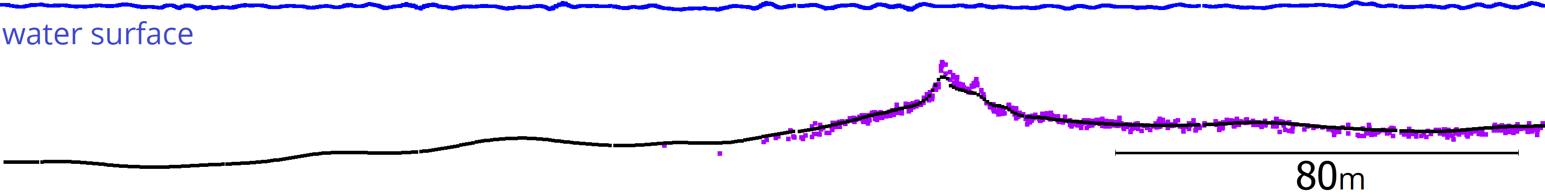
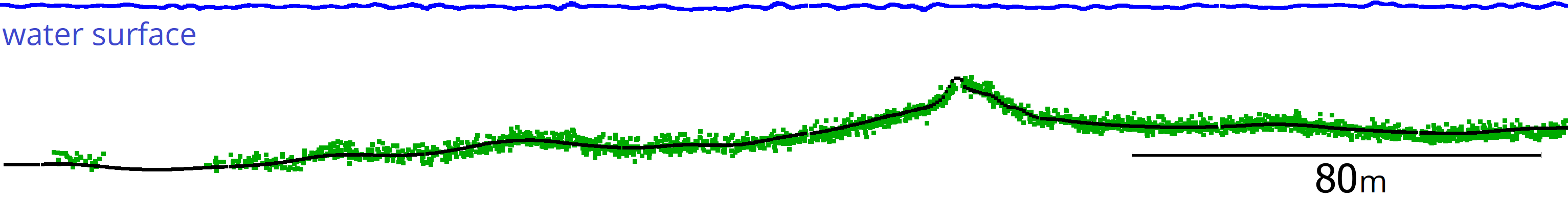
The cross section in Fig. 16 visually confirms both the good representation and the improved coverage of the seabed by the full-waveform stacking methods. Both the “hillock” (relatively centered) and the smaller ground waves (on the left) are clearly visible in the sigFWFS and volFWFS point clouds. Furthermore, the cross sections show that OWP, sigFWFS, and volFWFS exhibit a consistently even vertical scatter around the hydroacoustic measurement points. Additionally, the sigFWFS and volFWFS points display a larger vertical scattering compared to the OWP points. Section 5.2 contains quantitative analysis that supports these findings. Possible reasons for the scattering behavior discrepancies could result from differences in peak detectors and filtering methods utilized in the OWP processing. Applying water bottom models may result in reduced scattering behavior for sigFWFS and volFWFS point clouds.
5.2 Quantitative analysis of the results
A quantitative evaluation of the results is performed to confirm the good visual impressions from Figs. 15 and 16 and to better evaluate the potential of both full-waveform stacking methods for this ALB dataset. In the following, the results of the full-waveform processing are compared with the hydroacoustic measurements, and the accuracy and reliability are examined based on the height differences between the point clouds.
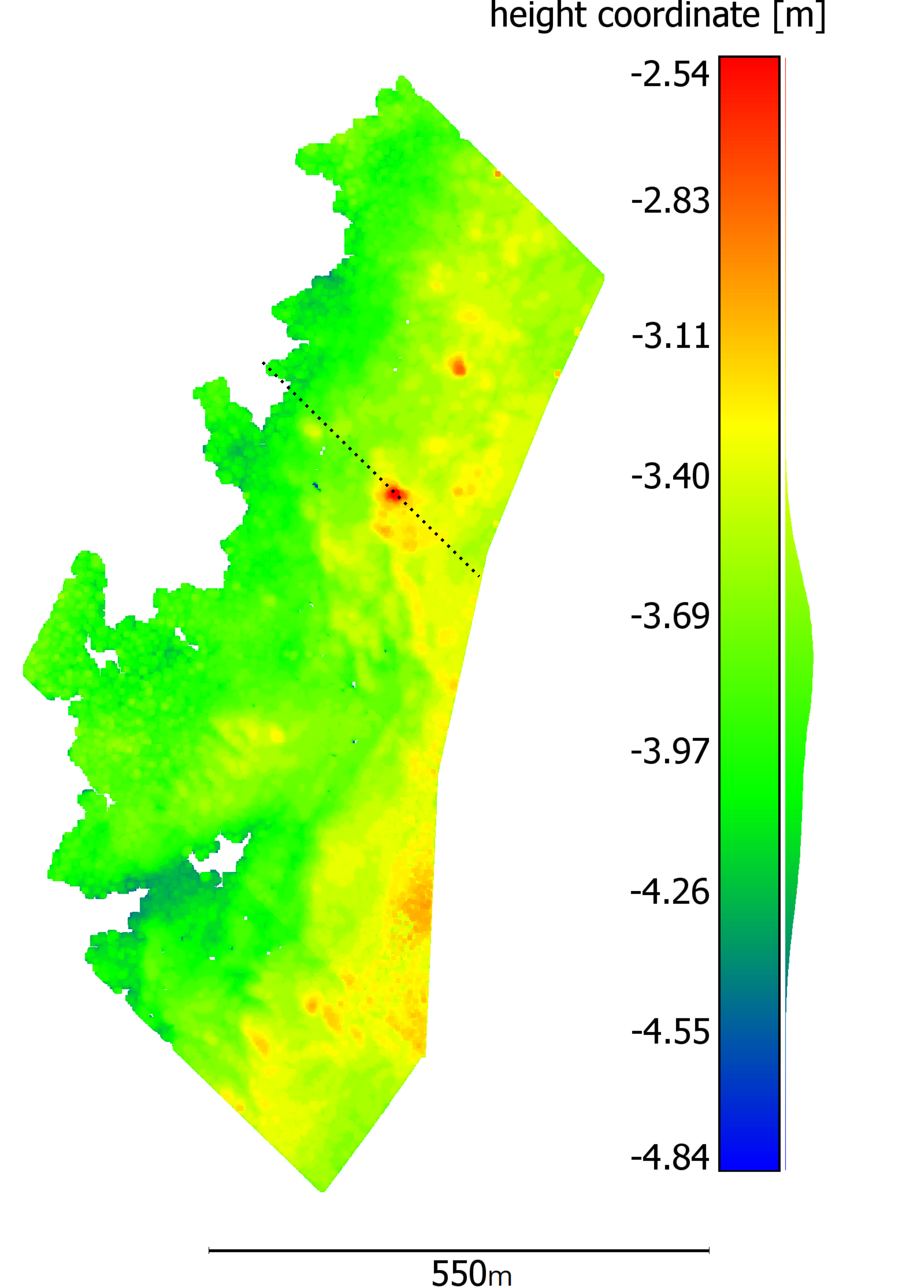
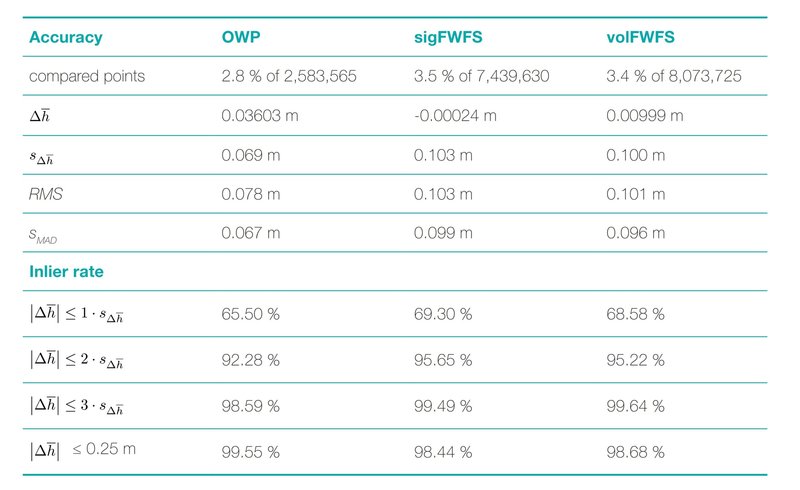
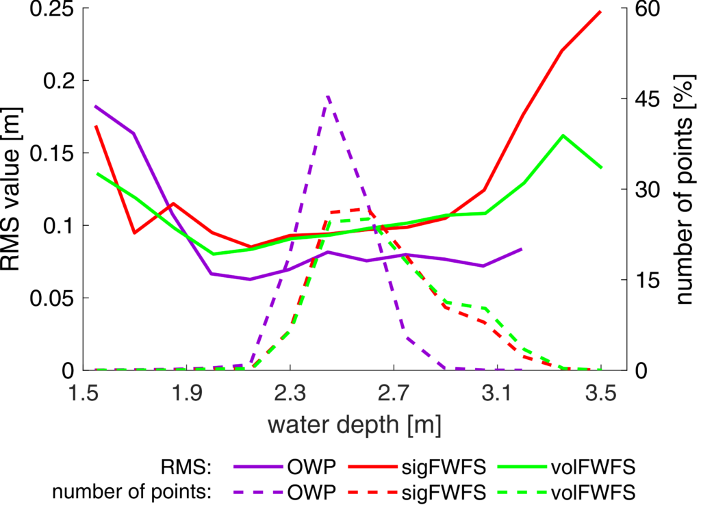
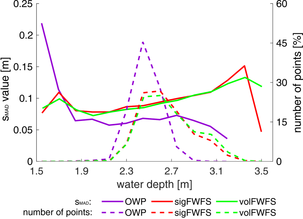
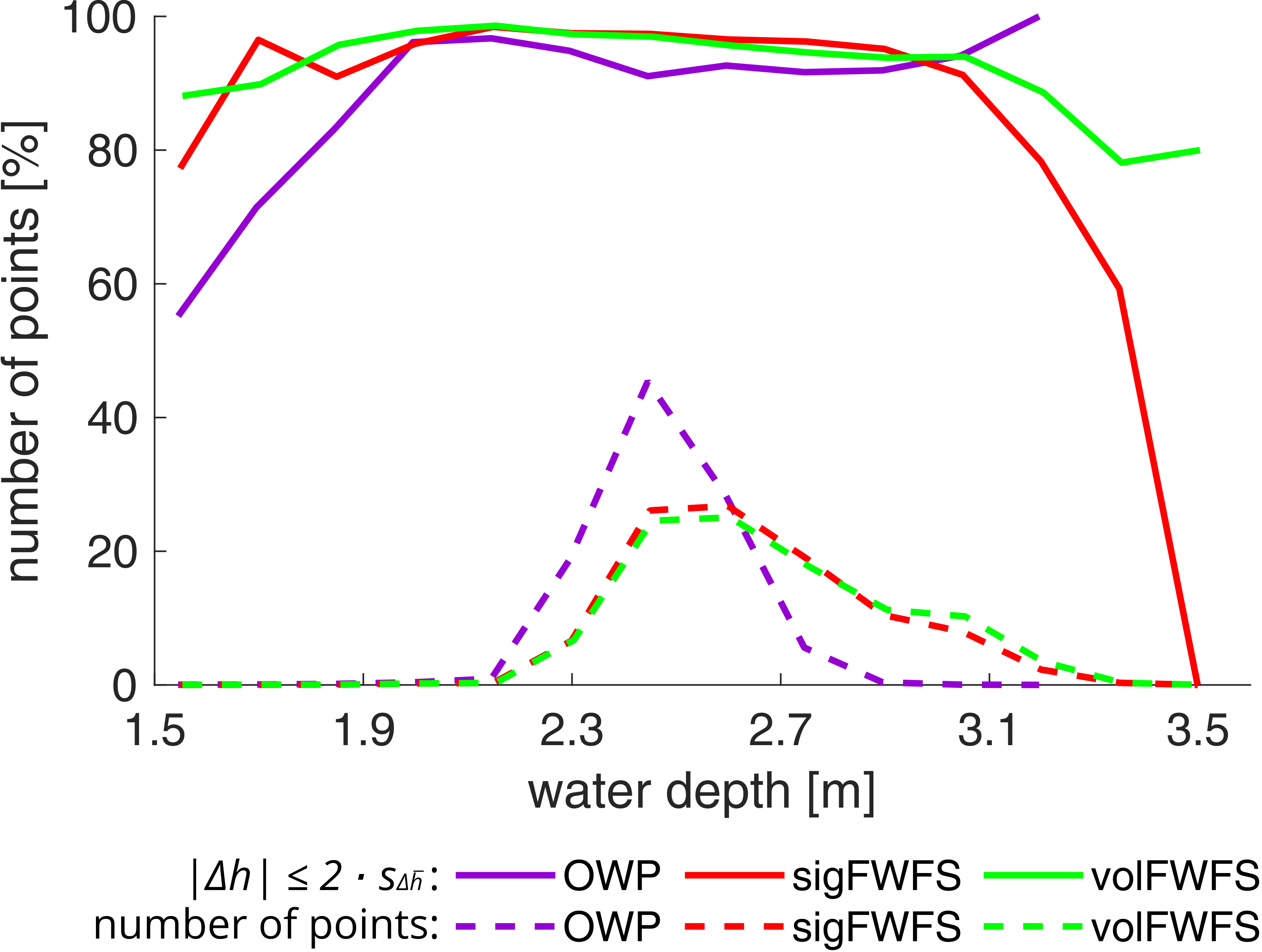
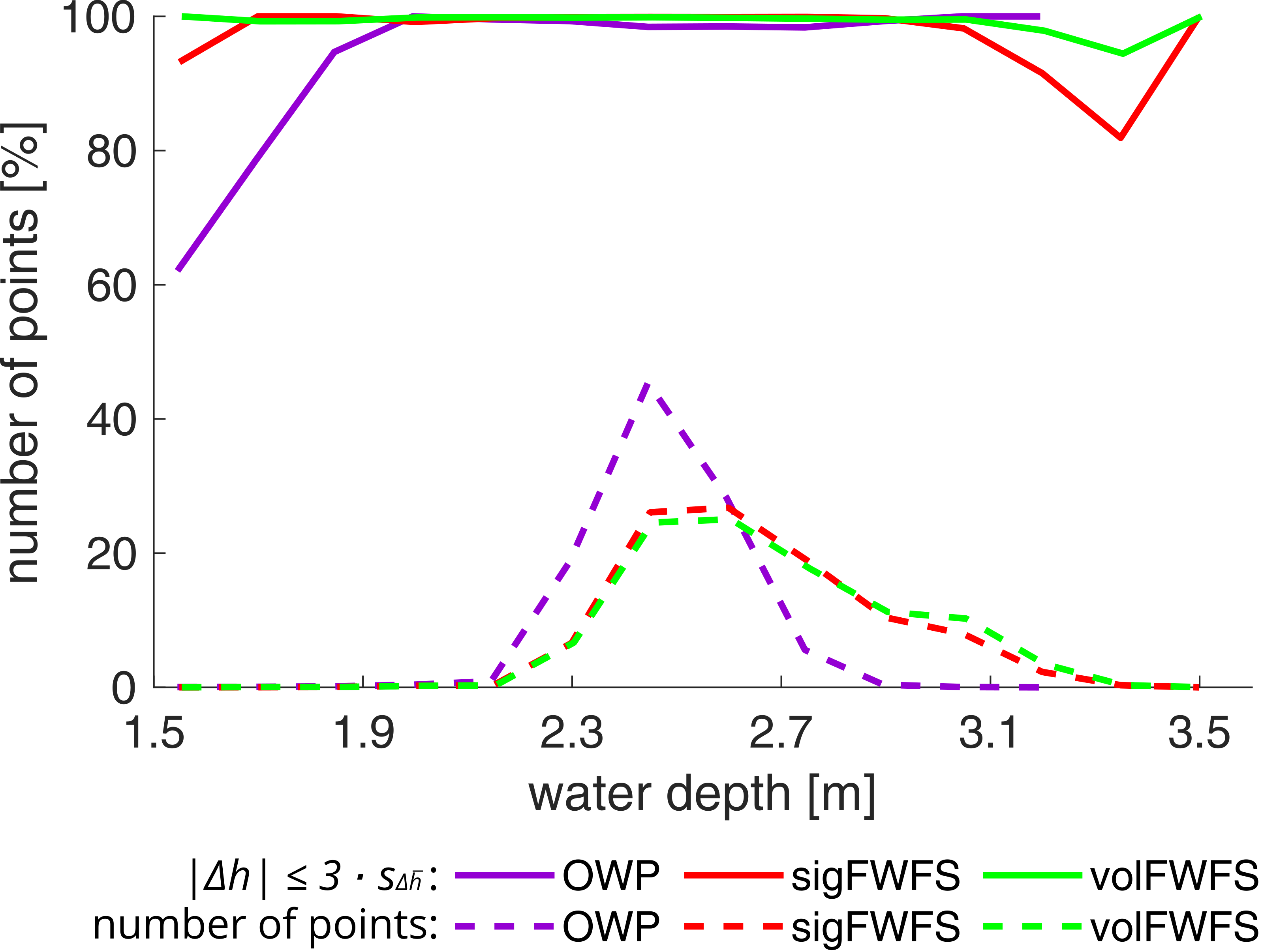
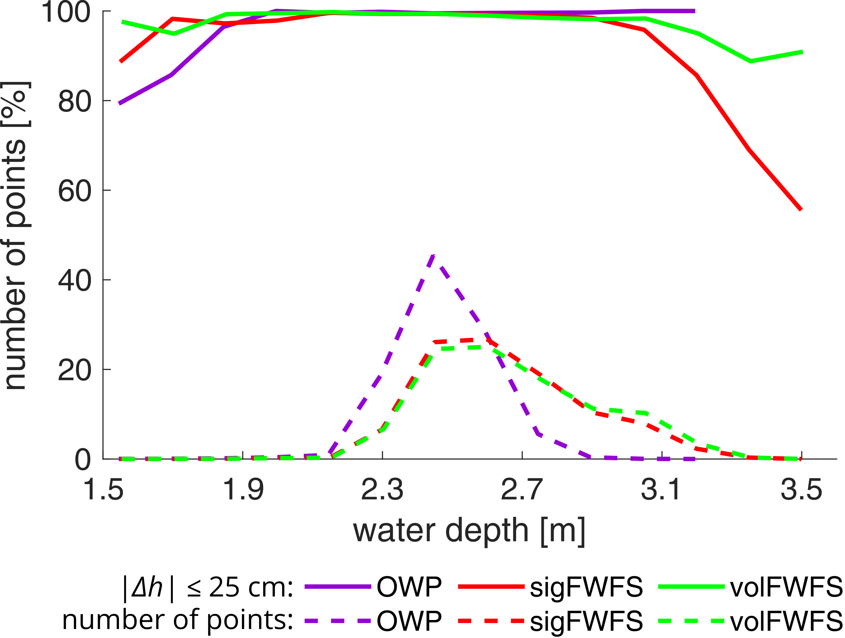
Fig. 17 shows the height differences for OWP, sigFWFS and volFWFS processing methods, with the sigFWFS differences appearing more inhomogeneous. The global accuracy values in Table 1 shows that more points were generated by the volFWFS and that these have a slightly higher compared to the hydroacoustic measurements. The other accuracy values (RMS, sMAD) vary by less than 1 cm between the full-waveform stacking methods. The RMS and sMAD values of the sigFWFS and volFWFS differ only slightly, implying that the systematic error seems to be minimal, which is also confirmed by the low . The OWP points have compared to the full-waveform stacking a better RMS and sMAD value but also a higher . Figs. 18a and 18b show the obtained accuracy values as a function of water depth, which are almost completely at a constant low level for water depths between 1.70 m and 3.50 m. The only exception is the RMS value of sigFWFS, which increases from 0.12 m to 0.25 m for water depths between 3.05 m and 3.50 m.
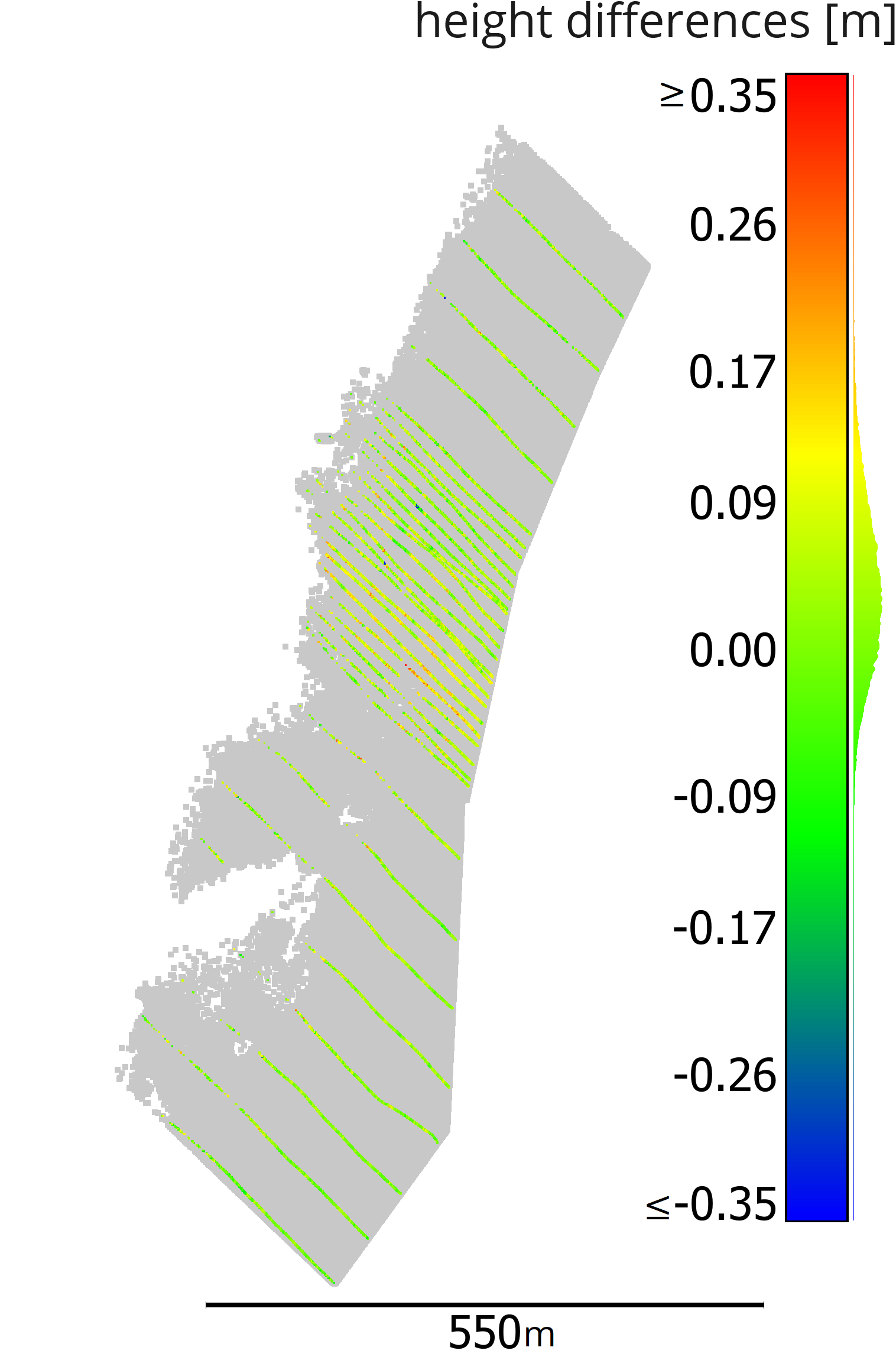
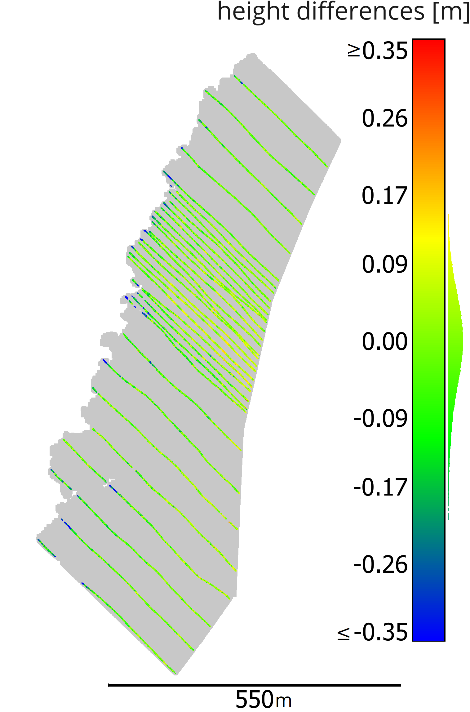
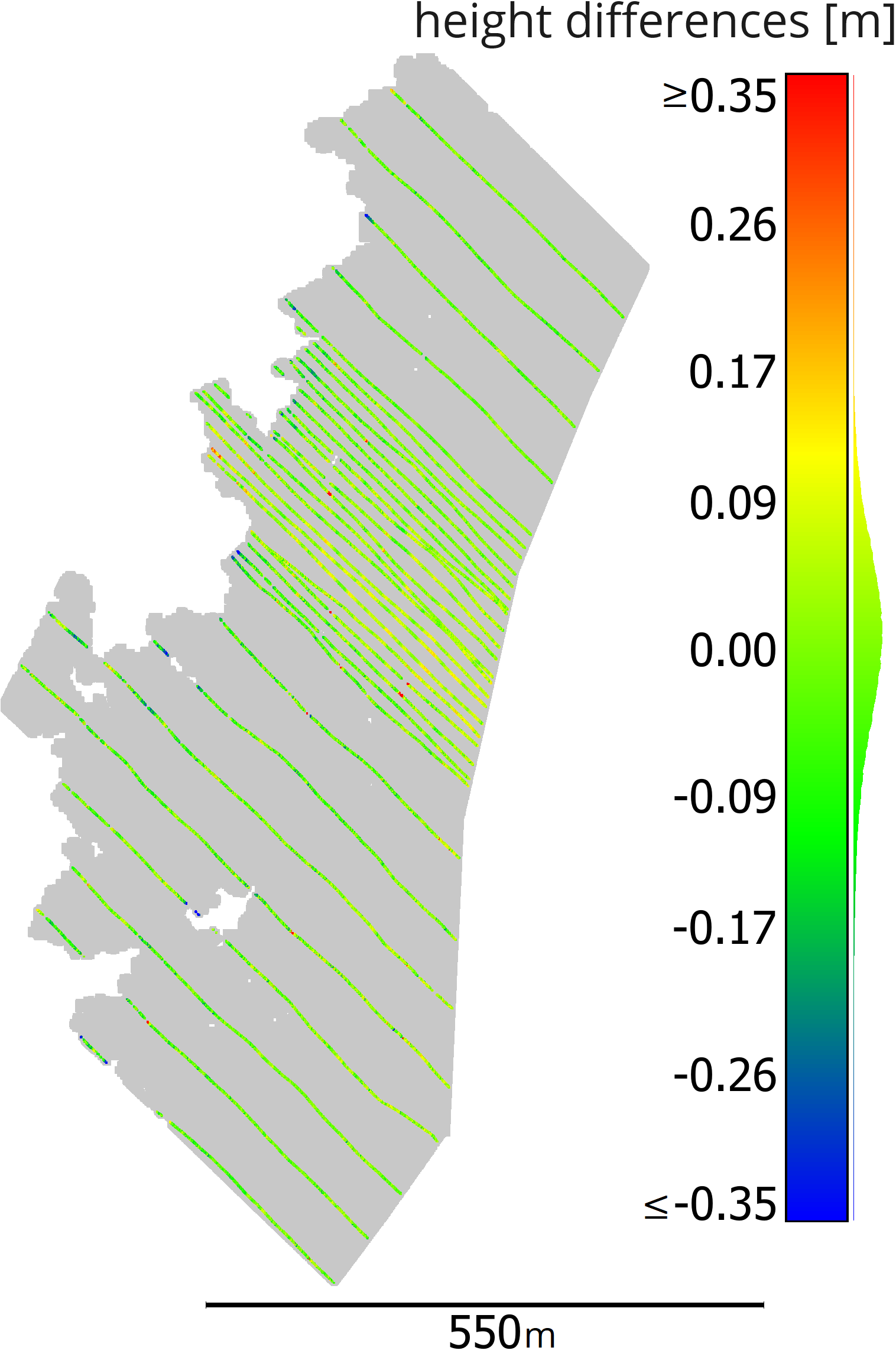
Fig. 17 Height differences of the resulting point clouds of the OWP processing and the two full-waveform stacking methods compared to the hydroacoustic profile measurements. The point clouds are color coded according to the height difference. Points with a positive height difference are underestimated and points with a negative height difference are overestimated.
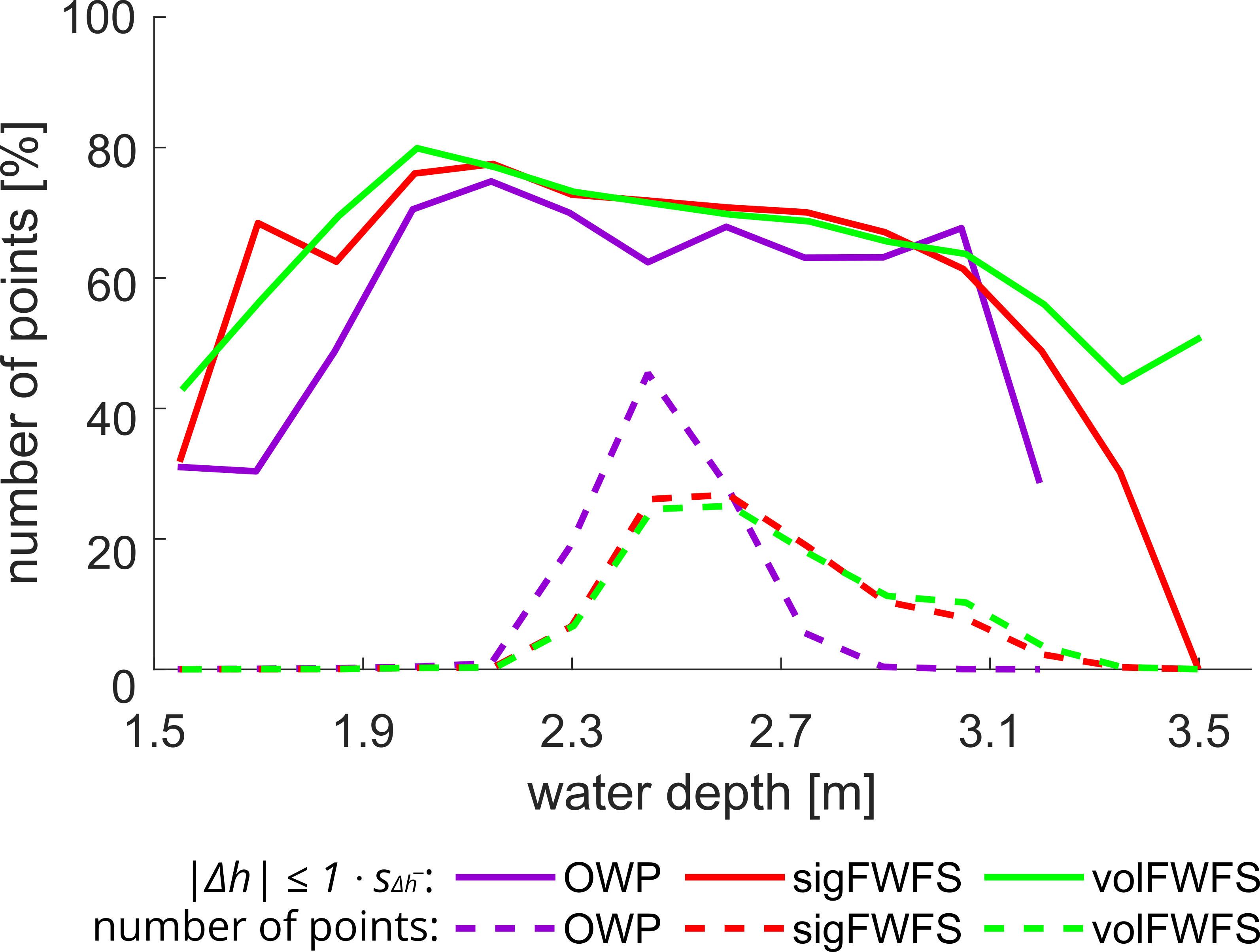
Regarding the global reliability values in Table 1, the inlier rate for all methods show very high values that differ only slightly from each other, except when  . The same can be observed for the inlier rates as a function of water depth (; Fig. 18c). The other inlier rates show a consistently good level for water depths between 1.70 m and 3.50 m, with the values for sigFWFS becoming visibly worse at water depths of 3.05 m and above (Figs. 18d to 18f). At a water depth of 3.20 m, 85.67 % of the points still have an absolute height difference ≤ 0.25 m, at 3.35 m there are still 69.05 %. The analysis of the accuracy and reliability of the obtained results shows that the seabed is well represented up to a water depth of about 3.20 m (sigFWFS) and 3.50 m (volFWFS) compared to the hydroacoustic measurements.

 ≤ 25 cm
Fig. 18 Plot of accuracy values and inlier rates. For (a) and (b), the solid lines refer to the left axis and the dashed line refers to the right axis. The values for OWP, sigFWFS and volFWFS can be found in Table 1.
5.3 Benefit of sigFWFS and volFWFS
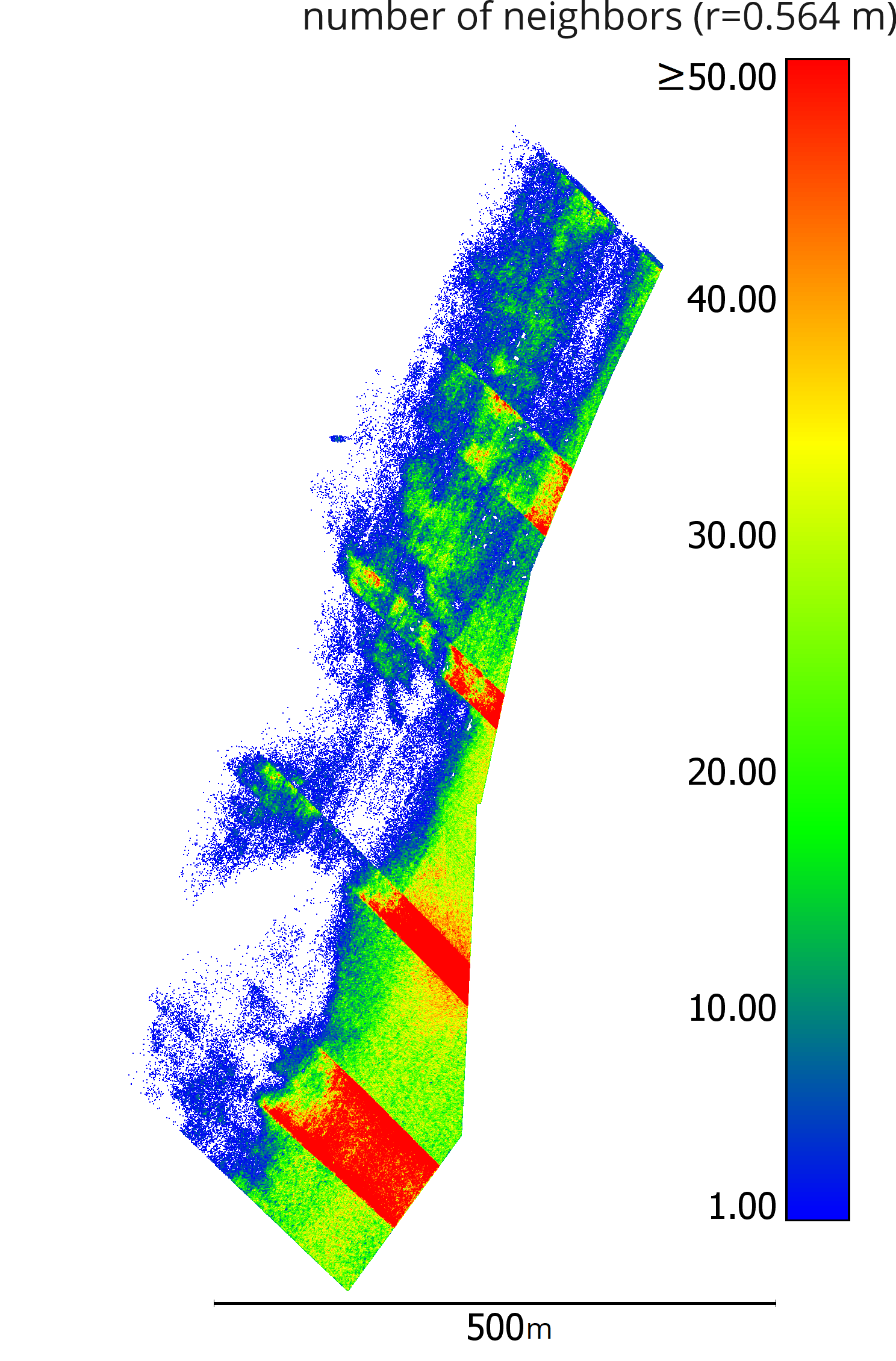
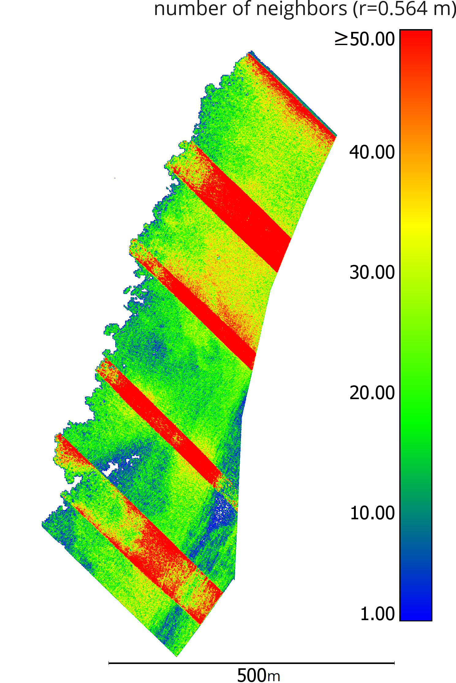
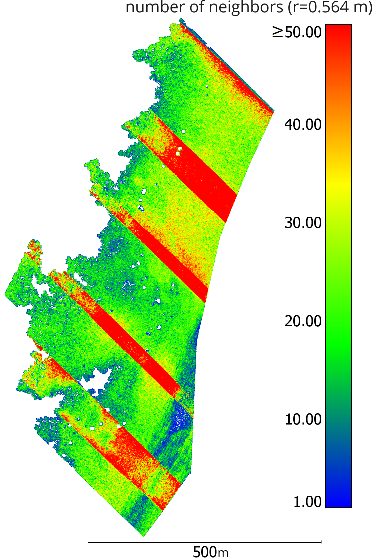
In this section, the benefit of full-waveform stacking methods compared to standard processing methods is investigated. For this purpose, it is obvious to analyze the increase in seabed covered and the analyzable water depth. In principle, both parameters are suitable for assessing the benefit, but the coverage increase is also strongly dependent on the characteristics of the seabed. In a study area with shallow depths and slightly sloping terrain, a significantly higher coverage increase can be expected than in an area with rapidly sloping terrain. In the point clouds (OWP and full-waveform stacking), a proportion of points have been attributed a depth that is deeper, and thus not necessarily representative of the entire point cloud. For the evaluation of the methods, the point density is introduced in addition to the two mentioned parameters. The point density for a point is here defined as the number of points within a maximum radius of 0.564 m (= 1 m2; 2D neighborhood). For a meaningful evaluation of the coverage increase, only the area of the points with a predefined point density is considered. The same applies to the water depth. For the investigated dataset, a minimum point density of 5 points/m2 is chosen. With such a point density, it should be possible to detect cubic objects with a side length of 1 m or more, which meets the IHO S-44 Special Order requirement for object detection.
Fig. 19 shows the point densities obtained by OWP, sigFWFS, and volFWFS. It can be clearly seen that in addition to the increase in area coverage, the point density was also increased in some areas. Based on the point density information, all points with a point density < 5 points/m2 were filtered out, the remaining points were projected into the XY plane and finally meshed. The meshed point cloud thus allows the determination of the area’s specification listed in Table 2. For a more meaningful area comparison, it is necessary to incorporate the OWP points between the study area and the land area of Amrum (Fig. 20). This results in a more realistic area increase of 11.4 % for sigFWFS and 14.6 % for volFWFS.
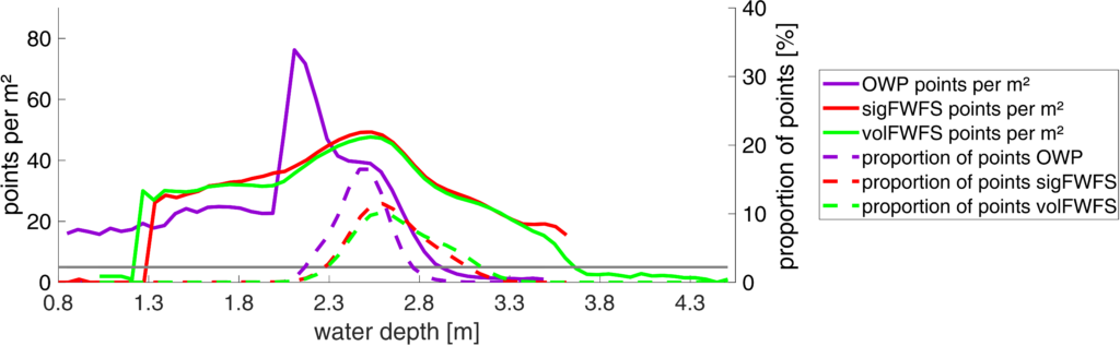
Fig. 21 shows the point density as a function of water depth. Taking into account the water surface from full-waveform stacking processing, the analyzable water depth achieved can be derived for the corresponding point density. The reachable water depths for a minimum point density of 5 points/m2 are shown in Table 2. The values may be overestimated due to the scattering of the bottom points (see sMAD).
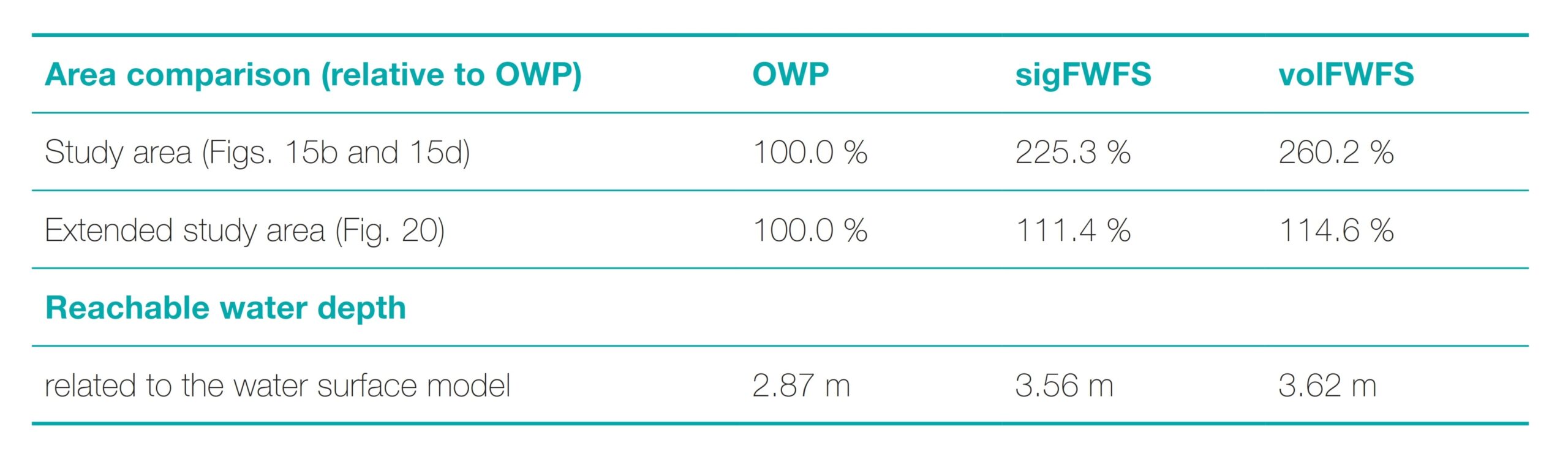
In summary, the analyzable water depth could be increased by 24 % for sigFWFS and by 26 % for volFWFS, resulting in a coverage increase of 11.4 % and 14.6 %, respectively, and a partial increase in point density.
A major advantage of full-waveform stacking processing is that basically a reprocessing of an existing ALB data is also possible, as long as they meet the requirements for full-waveform processing (OWP data with full-waveforms, full-waveform recording must contain water surface and seabed/riverbed without interruption, trajectory data). However, the processing of full-waveform stacking requires additional effort and therefore represents a complementary processing to the standard processing methods (OWP data). For time-optimized processing, full-waveform stacking should be used for selected areas where the OWP data reaches its limits or the point density becomes too low. In areas with sufficient point density, the OWP points already represent the seabed very well. Consequently, a hybrid point cloud is the best and most efficient solution for representing the entire seabed. This is especially recommended when processing ALB data with the volFWFS method, since the processing time and resources are many times higher than with sigFWFS due to the voxelization (mapping each sample of a full-waveform into voxel space).
6 Conclusion
This article shows the potential of full-waveform stacking techniques applied to marine ALB data. The two full-waveform stacking techniques sigFWFS and volFWFS are briefly introduced. In addition, a modification of both processing approaches is presented, which takes into account the actual water surface information and consequently the correction of the water surface underestimated by the green laser. Both full-waveform stacking approaches were applied to ALB data from the German Wadden Sea National Park. The results were evaluated with hydroacoustic measurements and the benefits in comparison to standard processing methods were discussed.
The analyzable water depth was increased by 24 % with the sigFWFS, resulting in a coverage increase of 11.4 %. With volFWFS, the water depth was increased by 26 %, resulting in a coverage increase of 14.6 %. The RMS value of 0.10 m (sigFWFS and volFWFS) as well as the high inlier rates of 98.44 % (sigFWFS) and 98.68 % (volFWFS) for points with a maximum height difference of 25 cm demonstrate the good accuracy and high reliability of the full-waveform stacking methods. It should be noted that the above quantitative statements apply only to the data set at hand. The results of the full-waveform stacking process depend on the following various factors, among others, and can vary accordingly:
- Water turbidity
- Water depth
- Submarine topography
- Sensor or sensor settings (e.g. beam divergence, field-of-view, laser pulse energy, point density)
This article has shown that with further developed and appropriate processing methods, additional information from the ALB measurement data can be extracted, thus the value of the ALB measurement data is increased. With respect to the research question formulated in Section 2, it can be concluded that the application of full-waveform stacking techniques to coastal ALB data can be beneficial in terms of increases the analyzable water depth and, consequently, improving the representation of the seabed.
Acknowledgements
The work presented was carried out as part of the R&D project “ALB-Nordsee – Laserbathymetrie in küstennahen Bereichen der Nordsee”, funded by the German Federal Maritime and Hydrographic Agency (BSH). We thank BSH for the opportunity to continue our research in LiDAR bathymetry. The data set acquired in the North Sea has contributed significantly to the further development of full-waveform stacking techniques. In addition, we thank the MILAN Geo-service GmbH for the very good cooperation in the preparation of the survey data.
References
An, L., Rignot, E., Millan, R., Tinto, K. and Willis, J. K. (2019). Bathymetry of Northwest Greenland using “Ocean Melting Greenland” (OMG) High-Resolution Airborne Gravity and other data. Remote Sensing, 11(2), 131. https://doi.org/10.3390/rs11020131
Bian, Z., Bai, Y., Douglas, W. S., Maher, A. and Liu, X. (2022). Multi-year planning for optimal navigation channel dredging and dredged material management. Transportation Research Part E-logistics and Transportation Review, 159, 102618. https://doi.org/10.1016/j.tre.2022.102618
Christiansen, L. (2021). Laser Bathymetry for Coastal Protection in Schleswig-Holstein. PFG–Journal of Photogrammetry, Remote Sensing and Geoinformation Science, 89(2), 183–189. https://doi.org/10.1007/s41064-021-00149-w
De Groot, S. (1986). Marine sand and gravel extraction in the North Atlantic and its potential environmental impact, with emphasis on the North Sea. Ocean Management, 10(1), 21–36. https://doi.org/10.1016/0302-184x(86)90004-1
Ellmer, W., Anderson, R., Flatman, A., Mononen, J., Olsson, U. and Öiås, H. (2014). Feasibility of laser bathymetry for hydrographic surveys on the Baltic Sea. The International Hydrographic Review, 12, 33–50. https://journals.lib.unb.ca/index. php/ihr/article/download/22840/26528
Fan, D., Li, S., Li, X., Yang, J. and Wan, X. (2020). Seafloor Topography Estimation from Gravity Anomaly and Vertical Gravity Gradient Using Nonlinear Iterative Least Square Method. Remote Sensing, 13(1), 64. https://doi.org/10.3390/rs13010064
Guenther, G. C. (1985). Airborne laser hydrography: system design and performance factors. Technical report, National Oceanic and Atmospheric Administration Rockville MD.
Guenther, G. C., Cunningham, A. G., LaRocque, P. E. and Reid, D. J. (2000). Meeting the accuracy challenge in airborne bathymetry. Technical report, National Oceanic Atmospheric Administration / NESDIS Silver Spring, MD.
Guo, X., Jin, X. and Jin, S. (2022). Shallow Water Bathymetry Mapping from ICESat-2 and Sentinel-2 Based on BP Neural Network Model. Water, 14(23), 3862. https://doi.org/10.3390/w14233862
Hampel, F. R. (1974). The Influence Curve and its Role in Robust Estimation. Journal of the American Statisti-cal Association, 69(346), 383–393. https://doi.org/10.1080/01621459.1974.10482962
Hartmann, K., Reithmeier, M., Knauer, K., Wenzel, J., Kleih, C. and Heege, T. (2022). Satellite-derived bathymetry online. The International Hydrographic Review, 28, 53–75. https://doi.org/10.58440/ihr-28-a14
Hecht, H. (2023). Hydrographic GIS. The International Hydrographic Review, 29(1), 158–162. https://doi.org/10.58440/ihr-29-a11
Hendriks, H., Van Prooijen, B. C., Aarninkhof, S. and Winterwerp, J. C. (2020). How human activities affect the fine sediment distribution in the Dutch Coastal Zone seabed. Geomorphology, 367, 107314. https://doi.org/10.1016/j.geomorph.2020.107314
Höhle, J. (1971). Zur Theorie und Praxis der Unterwasser-Photogrammetrie. PhD-Thesis, Universität Karlsruhe (TH).
IHO-IOC (2018). The IHO-IOC GEBCO Cook Book. IHO Publication B-11, International Hydrographic Organization, Monaco, 416 pp. IOC Manuals and Guides 63, Intergovernmental Oceanographic Commission, France, 429 pp. https://doi.org/10.58440/iho-b-11
IHO (2020). Standards for Hydrographic Surveys (6th ed.). IHO Special Publication S-44, International Hydrographic Organization, Monaco.
Jonas, M. (2023). New horizons for hydrography. The International Hydrographic Review, 29(1), 16–24. https://doi.org/10.58440/ihr-29-a01
Korhonen, J. (2014). Baltic Sea Hydrographic Re-Survey Scheme “To ensure that safety of navigation is not endangered by inadequate source information”. The International Hydrographic Review, 12, 7–20.
Kubicki, A., Manso, F. and Diesing, M. (2007). Morphological evolution of gravel and sand extraction pits, Tromper Wiek, Baltic Sea. Estuarine Coastal and Shelf Science, 71(3–4), 647–656. https://doi.org/10.1016/j.ecss.2006.09.011
Laporte, J., Dolou, H., Avis, J. and Arino, O. (2023). Thirty years of satellite derived bathymetry – The charting tool that hydrographers can no longer ignore. The International Hydrographic Review, 29(1), 170–184. https://doi.org/10.58440/ihr-29-a20
Letard, M., Collin, A., Corpetti, T., Lague, D., Pastol, Y., Gloria, H., James, D. and Mury, A. (2021). Classification of coastal and estuarine ecosystems using full-waveform topo-bathymetric lidar data and artificial intelligence. OCEANS 2021: San Diego– Porto. https://doi.org/10.23919/oceans44145.2021.9705797
Litman, R., Korman, S., Bronstein, A. and Avidan, S. (2015). Inverting RANSAC: Global model detection via inlier rate estimation. Proceedings of the 2015 IEEE Conference on Computer Vision and Pattern Recognition (CVPR). https://doi.org/10.1109/cvpr.2015.7299161
Lurton, X. (2002). An introduction to underwater acoustics: principles and applications. Springer Science & Business Media.
Mader, D., Richter, K., Westfeld, P., Weiss, R. and Maas, H.-G. (2019). Detection and extraction of water bottom topography from laserbathymetry data by using full-waveform-stacking techniques. The International Archives of the Photogrammetry, Remote Sensing and Spatial Information Sciences, XLII-2/ W13, 1053–1059. https://doi.org/10.5194/isprs-archives-xlii-2-w13-1053-2019
Mader, D., Richter, K., Westfeld, P. and Maas, H.-G. (2021). Potential of a non-linear Full-Waveform stacking technique in airborne LiDAR bathymetry. PFG – Journal of Photogrammetry, Remote Sensing and Geoinformation Science, 89(2), 139–158. https://doi.org/10.1007/s41064-021-00147-y
Mader, D., Richter, K., Westfeld, P. and Maas, H.-G. (2023). Volumetric Nonlinear Ortho Full-Waveform Stacking in Airborne LiDAR Bathymetry for Reliable Water Bottom Point Detection in Shallow Waters. ISPRS Journal of Photogrammetry and Remote Sensing, 204, 145–162. https://doi.org/10.1016/j.isprsjprs.2023.08.014
Mandlburger, G., Pfennigbauer, M. and Pfeifer, N. (2013). Analyzing near water surface penetration in laser bathymetry – A case study at the River Pielach. ISPRS Annals of the Photogrammetry, Remote Sensing and Spatial Information Sciences, II-5/W2, 175–180. https://doi.org/10.5194/isprsannals-ii-5-w2-175-2013
Mandlburger, G. (2020). A Review of Airborne Laser Bathymetry for Mapping of Inland and Coastal Waters. Hydrographische Nachrichten, 116, 6–15. https://doi.org/10.23784/HN116-01
Mandlburger, G. (2021). Bathymetry from Images, LiDAR and Sonar: From Theory to Practice. PFG–Journal of Photogrammetry, Remote Sensing and Geoinformation Science, 89(2), 69–70.
Mandlburger, G. (2022). A Review of Active and Passive Optical Methods in Hydrography. The International Hydrographic Review, 28, 8–52. https://doi.org/10.58440/ihr-28-a15
Mielck, F., Hass, H. C., Michaelis, R., Sander, L., Papenmeier, S. and Wiltshire, K. H. (2018). Morphological changes due to marine aggregate extraction for beach nourishment in the German Bight (SE North Sea). Geo-marine Letters, 39(1), 47–58. https://doi.org/10.1007/s00367-018-0556-4
Pan, Z., Glennie, C. L., Fernandez-Diaz, J. C., Legleiter, C. J. and Overstreet, B. T. (2016). Fusion of LIDAR orthowaveforms and hyperspectral imagery for shallow river bathymetry and turbidity estimation. IEEE Transactions on Geoscience and Remote Sensing, 54(7), 4165–4177. https://doi.org/10.1109/tgrs.2016.2538089
Pandian, P. K., Ruscoe, J. P., Shields, M. A., Side, J. C., Harris, R. E., Kerr, S. A. and Bullen, C. (2009). Seabed habitat mapping techniques: an overview of the performance of various systems. Mediterranean Marine Science, 10(2), 29–44. https://doi.org/10.12681/mms.107
Parrish, C., Magruder, L. A., Neuenschwander, A. L., Forfinski-Sarkozi, N. A., Alonzo, M. and Jasinski, M. F. (2019). Validation of ICESat-2 ATLAS Bathymetry and Analysis of ATLAS’s Bathymetric Mapping Performance. Remote Sensing, 11(14), 1634. https://doi.org/10.3390/rs11141634
Pe’eri, S., Parrish, C., Azuike, C., Alexander, L. and Armstrong, A. (2014). Satellite remote sensing as a reconnaissance tool for assessing nautical chart adequacy and completeness. Marine Geodesy, 37(3), 293–314. https://doi.org/10.1080/01490419.2014.902880
Pfennigbauer, M., Rieger, P., Studnicka, N. and Ullrich, A. (2009). Detection of concealed objects with a mobile laser scanning system. In Monte D. Turner and Gary W. Kamerman (Eds.), Laser Radar Technology and Applications XIV, Proceedings of SPIE, 7323, 51–59. https://doi.org/10.1117/12.828293
Pfennigbauer, M. and Ullrich, A. (2010). Improving quality of laser scanning data acquisition through calibrated amplitude and pulse deviation measurement. In Monte D. Turner and Gary W. Kamerman (Eds.), Laser Radar Technology and Applications XV, SPIE proceedings, 7684, 463–472. https://doi.org/10.1117/12.849641
Plenkers, K., Ritter, J. and Schindler, M. (2013). Low signalto-noise event detection based on waveform stacking and cross-correlation: application to a stimulation experiment. Journal of Seismology, 17(1), 27–49. https://doi.org/10.1007/s10950-012-9284-9
Ratick, S. J., Wei, D. and Moser, D. A. (1992). Development of a reliability based dynamic dredging decision model. European Journal of Operational Research, 58(3), 318–334. https://doi.org/10.1016/0377-2217(92)90063-f
Roncat, A. and Mandlburger, G. (2016). Enhanced detection of water and ground surface in airborne laser bathymetry data using waveform stacking. EGU General Assembly Conference Abstracts, 18, 17016.
Sachs, L. (1982). Applied Statistics: A Handbook of Techniques. Springer-Verlag.
Sandwell, D. T., Müller, R. D., Smith, W. H. F., Garcia, E. S. M. and Francis, R. (2014). New global marine gravity model from CryoSat-2 and Jason-1 reveals buried tectonic structure. Science, 346(6205), 65–67. https://doi.org/10.1126/science.1258213
Smith, W. H. F. and Sandwell, D. T. (1994). Bathymetric prediction from dense satellite altimetry and sparse shipboard bathyme ry. Journal of Geophysical Research, 99(B11), 21803–21824. https://doi.org/10.1029/94jb00988
Stilla, U., Yao, W., & Jutzi, B. (2007). Detection of weak laser pulses by full waveform stacking. The International Archives of the Photogrammetry, Remote Sensing and Spatial Information Sciences, 36, 25–30.
Wölfl, A., Snaith, H., Amirebrahimi, S., Devey, C. W., Dorschel, B., Ferrini, V. L., Huvenne, V., Jakobsson, M. et al. (2019). Seafloor Mapping – The Challenge of a Truly Global Ocean Bathymetry. Frontiers in Marine Science, 6, 283. https://doi.org/10.3389/fmars.2019.00283
Authors’ biographies

Dr.-Ing. David Mader is a PostDoc at the Institute of Photogrammetry and Remote Sensing at the TU Dresden and research associate at the Center for UAV Photogrammetry. In 2022, he received his Ph.D. on novel methods for the analysis of airborne LiDAR bathymetry data. In this context, he developed full-waveform stacking techniques for the detection of weak water-bottom echoes in airborne LiDAR bathymetry. His research focuses on improved derivation of water bottom topography from airborne LiDAR bathymetry data, enabling an efficient monitoring of shallow water areas of rivers, lakes and oceans.

Dr.-Ing. Katja Richter is a research assistant at the Institute of Photogrammetry and Remote Sensing at the TU Dresden. In 2018, she received her Ph.D. on the topic “Analysis of full-waveform airborne laser scanner data for volumetric representation in environmental applications”. Her research interests include the development of novel data analysis techniques in airborne LiDAR bathymetry with a particular focus on deriving high spatial resolution water turbidity parameters and increasing the accuracy potential of the measuring method.

Dr.-Ing. Patrick Westfeld graduated as a geodesist in 2005 from TU Dresden (Germany). He conducted research in the fields of photogrammetry and laser scanning and completed his PhD in 2012 on geometric-stochastic modeling and motion analysis. Since 2017, Dr Westfeld heads R&D at BSH, the German Federal Maritime and Hydrographic Agency. The activities of his section range from conceptual issues pertaining to hydroacoustic and imaging sensor technologies, sensor integration and modeling, algorithmic development up to application-specific implementation and practical transfer in the production environment.

Jean-Guy Nistad holds an Engineering degree from McGill University (Canada), a graduate diploma in GIS from Université du Québec à Montréal (Canada) and a graduate degree in hydrography from HafenCity University Hamburg. From 2007 to 2013 he worked for the Interdisciplinary Centre for the Development of Ocean Mapping (Canada) where he gained most of his expertise in hydrographic surveying. Since 2016, he has been employed by BSH, the Federal Maritime and Hydrographic Agency of Germany, in the section “Geodetic-hydrographic Techniques and Systems”. His current tasks include research & development, technical support on multibeam issues and hydrographic teaching.

Prof. Dr. sc. techn. habil. Hans-Gerd Maas is Professor for Photogrammetry at TU Dresden, Germany. His research is dedicated to the development of efficient measurement solutions and processing algorithms with special emphasis on environmental monitoring tasks in forestry, glaciology, and hydrology. One focus of the Photogrammetry Group at TU Dresden is on novel monitoring and forecasting technologies for cooperative risk management of hydrological extreme events, 3D monitoring for bank protection measures, and the improvement of the application potential of LiDAR bathymetry as well as the necessary assurance of the accuracy and reliability of LiDAR bathymetry data.