1 Introduction

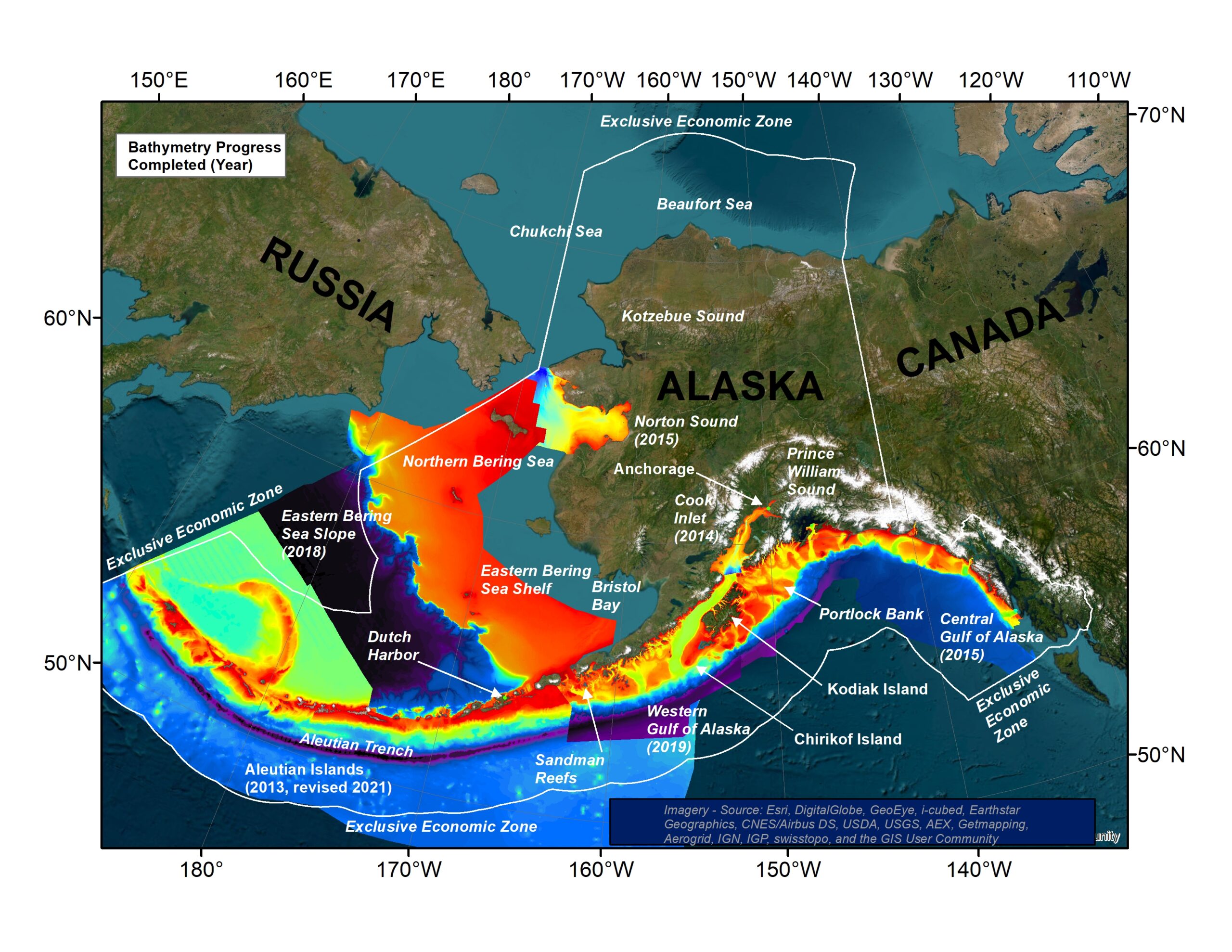
Charting the seas¹ and managing fisheries² within the United States (U.S.) Exclusive Economic Zone (EEZ) are two important responsibilities of the U.S. Department of Commerce’s National Oceanic and Atmospheric Administration (NOAA). These closely linked activities are challenging to conduct in the EEZ off of the U.S. state of Alaska due to its remoteness, vastness, stormy oceans, complicated seafloor topography, and abundance of federally managed fishery resources (for location see Fig. 1). Alaska’s EEZ would be the tenth largest in the world if Alaska was considered to be its own country. Alaska has the lowest population density of all U.S. states³ and is also one of the least populated, with over half of its citizens living in or near Anchorage, its largest city. Thus, many areas are uninhabited or only occupied by small communities, such that there are large hydrographic gaps outside of thoroughly mapped marine transit corridors and commercially important ports. Here we define gaps as areas where we were unable to find any bathymetry data. Harsh weather conditions, including hurricane-strength storms, substantial seasonal sea ice, large tides, strong currents, and shallow, rocky areas that are too dangerous to approach, such as the Sandman Reefs, and areas exceeding 7,000 m in depth, such as the Aleutian Trench make work difficult both for hydrographers and fisheries researchers. Alaska consistently has the largest commercial catch by weight and value among all U.S. states and its port of Dutch Harbor consistently tops the list of annual landings⁴. These valuable and economically important fisheries often occur in distant, poorly mapped areas of Alaska but require a great deal of oversight and scientific knowledge to be sustainable.

2 Study area’s utility of navigational charts

Alaska navigational charts, often produced at a scale of 1:100,000 by NOAA’s National Ocean Service (NOS), are indispensable tools for the safe conduct of commercial fisheries and research activities of fishery biologists at NOAA’s National Marine Fisheries Service (NMFS). The fishing industry’s ability to find target species, avoid bycatch species, and to prevent gear damage or loss because of steep, hard, and rough seafloor can often require bathymetry at a much finer scale than is available from the charts. Since much of the commercial fishing activity occurs in areas that are not well-mapped by NOS, the industry has been utilizing tools such as Terrain Builder by ECC Globe⁵, Seabed Mapping in Olex⁶, and Fishing Workspace in TimeZero⁷ to create independent compilations or to combine their soundings with colleagues to produce group compilations such as that of the Alaska Longline Fishermen’s Association⁸. NMFS’s Alaska Fisheries Science Center (AFSC) has also used the NOS navigational charts to design and execute various fishery-independent bottom trawl surveys, as their survey stations and strata are partially defined by depth, and their estimates of biomass and population are also dependent upon depth. The AFSC bottom trawl surveys range from the nearshore to a maximum depth of ~ 80 m in the Northern Bering Sea (Lauth et al., 2019), 200 m in the eastern Bering Sea shelf (Lauth et al., 2019), 500 m in the Aleutian Islands (von Szalay & Raring, 2020), 1,000 m in the Gulf of Alaska (von Szalay & Raring, 2016), and 1,200 m in the eastern Bering Sea Slope (Hoff, 2016), generally exceeding the shallower mapping focus of the NOS navigational charts. Spatial modeling of the distribution and abundance of numerous fish and invertebrate species, an important analytical method conducted by staff at NMFS, is also highly dependent on better seafloor maps because bathymetry and bathymetric derivatives are the most important descriptive variables (e.g., Sigler et al., 2015; Laman et al., 2017; Turner et al., 2017; Rooney et al., 2018). The bottom trawl surveys and modeling exercises also require bathymetric data at a scale larger than the existing navigational charts.

3 Background for improving bathymetric knowledge

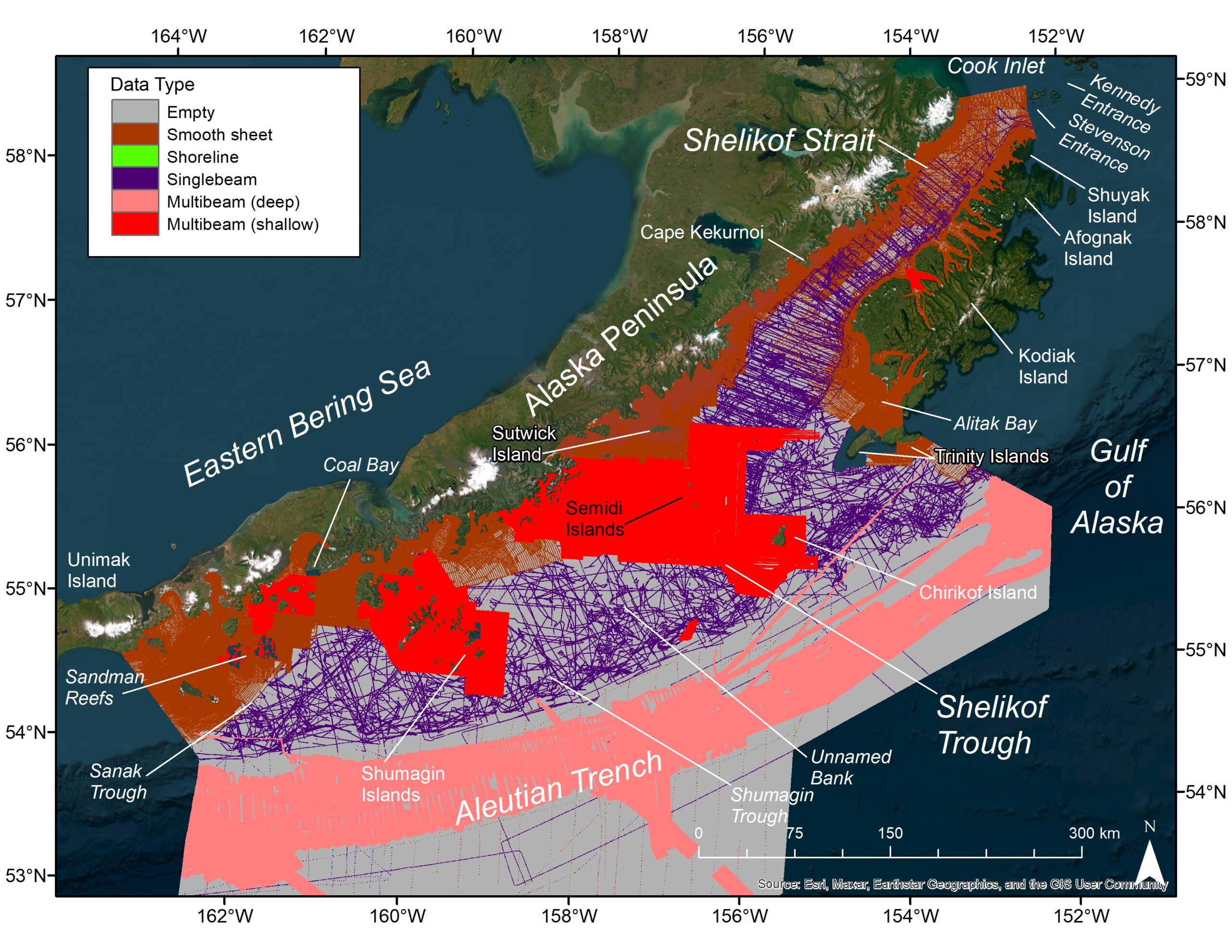
To meet the needs of NMFS research for managing the fishing industry, staff at NMFS’s AFSC have been creating 32-bit, floating-point bathymetry rasters (allowing decimal places and negative values) mostly from digitized data of NOS’s pre-chart hydrographic cruises, the smooth sheets (also known as Hydrographic or H-sheets), an online and free but unproofed source of bathymetry, often at a scale of 1:20,000. Here we define raster as a generic term for a continuous surface of equal sized squares and recognize that others use the term “grid”. In Alaska, many early smooth sheet cruises were conducted in the 1930s–1950s, so some users may suspect they are out of date and outclassed by the navigational charts, which are constantly being updated and republished. Unfortunately, this suspicion is due to a lack of understanding that these recent NOS charts are just lower resolution versions of these older smooth sheet data sets, often without any bathymetric updates, but include newer navigational information (buoys, lights, sea lanes, etc.) and newer publication dates. As a result, AFSC staff have developed methods of proofing and correcting digitization errors of these old smooth sheet data sets (Zimmermann and Benson, 2013), combining them with other sometimes non-hydrographic data sources, converting the data points into Triangulated Irregular Networks (TINs) and then into bathymetry rasters. These bathymetry rasters include the Aleutian Islands (AI: Zimmermann et al., 2013; Zimmermann & Prescott, 2021a, 2021b), Cook Inlet (CI: Zimmermann & Prescott, 2014), Norton Sound (NS: Prescott & Zimmermann, 2015), the Central Gulf of Alaska (CGOA: Zimmermann & Prescott, 2015), the Eastern Bering Sea Slope (EBSS: Zimmermann & Prescott, 2018), and the Western Gulf of Alaska (WGOA: Zimmermann et al., 2019b), all published at a horizontal resolution of 100 m except for Cook Inlet, which was published at 50 m (Fig. 1).

GEBCO (the General Bathymetric Chart of the Oceans organization) was founded in Monaco in 1903 to create the authoritative map of the world’s oceans, but with just a few thousand soundings available for the first edition. After over a century of periodically updated but still incomplete newer editions, GEBCO hosted the “Forum for Future Ocean Floor Mapping” in Monaco in 2016⁹ to develop a plan to improve the data support from 18 % to 100 % of their grid cells (GEBCO prefers the term “grid”) while also improving the resolution of the 30 arc-second (~ 1 km) grid cells to 100 m to 800 m, depending on depth (Mayer et al., 2018). At GEBCO’s 2017 Symposium¹⁰, this new effort was announced as “The Nippon Foundation – GEBCO Seabed 2030 Project”¹¹ and later published as a Concept Paper (Mayer et al., 2018). GEBCO’s new initiative was formally endorsed as a Decade Action of the United Nations Decade of Ocean Science for Sustainable Development.

Seabed 2030 divided the world’s oceans into four Regional Data Assembly Coordination Centers (RDACC¹²), and the AFSC regional bathymetry compilations of Alaska fell within the confines of the Arctic and North Pacific RDACC¹³, providing a geographic connection between the well-established IBCAO (International Bathymetric Chart of the Arctic Ocean) compilation (Jakobsson et al., 2020) and a new focus area of the North Pacific Ocean. AFSC staff had also previously been contributing these Alaska EEZ compilations to GEBCO’s global map (Weatherall et al., 2015), which is now being updated annually, most recently at a resolution of 15 arc-seconds (~ 245 m west to east, ~ 460 m north to south in the Gulf of Alaska) (e.g., GEBCO_2022 grid: GEBCO Bathymetric Compilation Group 2022, 2022).

Much of the GEBCO and Seabed 2030 discussions revolve around discovering new sources of archived or ongoing data collections, processing and incorporating data sets, and deciding where to conduct seafloor mapping expeditions. An offshoot of GEBCO – Map the Gaps¹⁴ – was founded to facilitate these discussions, provide mapping expertise to expeditions, and to host an annual symposium as collecting bathymetry data is often extremely expensive, and the costs to map unexplored ocean areas greatly exceed the funds available to support such efforts.

As a guide for future mapping work in Alaska, the AFSC Alaska regional bathymetry compilations can be too large (~ 2 GB) to work with easily, and they do not show which raster cells are supported by actual soundings and which cells are populated by interpolation. Although AFSC staff have also published tables listing various bathymetry research cruises, and maps showing the spatial distribution of these data sets, there is no simple, small, comprehensive guide available for future mapping work. Thus, we re-analyzed the source data of the AFSC staff regional bathymetry compilations, creating Type Identifier Grids (TIDs, also known as Source Identifier Grids¹⁵), a practice commonly conducted at GEBCO, to show which AFSC raster cells are supported by actual soundings, the type and quality of supporting data, and where the gaps are, to provide guidance for mapping the gaps of Alaska by 2030.

4 Methodology

In a Geographic Information System (GIS), we reviewed the data sources for the published Alaska regional bathymetry maps as well as other data sets that were not incorporated before the publication date. The data sources were grouped into five general types, listed here in general order of increasing quality: smooth sheets, digitized shorelines of the smooth sheets, singlebeam, deep water multibeam, and shallow water multibeam (including LiDAR or Light Detection and Ranging). All GIS work was performed in ArcMap (v.10.7.1, ESRI: Environmental Systems Research Institute, Redlands, CA). Unincorporated bathymetry data sets were plotted to determine their spatial extent in comparison to each other and previously incorporated data sets.

4.1 Smooth sheets

Smooth sheets mostly consist of thousands of soundings in units of fathoms, or sometimes feet, that are represented as positive numbers – deeper than the tidal datum of MLLW (Mean Lower Low Water), which is defined as zero depth. Soundings were originally conducted with lead lines but switched to fathometers, an early version of singlebeam echosounder, in the 1930s. Inshore smooth sheets may also include numerous noteworthy cartographic features, especially those that could interfere with safe navigation. Some of these cartographic features, such as rocks (submerged, awash, or always underwater), islets, and rocky reefs, may have depths or elevations associated with them. Depths or elevations from all of these cartographic features were included with the smooth sheet soundings, when possible, although the focus was on proofing and editing the soundings. Smooth sheet navigation was generally controlled by visual observation of triangulation station signals, with soundings carefully corrected by observed tides. These surveys were mostly limited to shallow and nearshore areas and often produced at large scales such as 1:20,000.

4.2 Shorelines

Smooth sheets also have ground-truthed versions of the Topographic or T-sheet shorelines. While technically shorelines are at an elevation (at MHW or Mean High Water above the MLLW datum of the smooth sheets) rather than a depth, they are represented on the same vertical scale of the smooth sheet depths, but as negative values. These shorelines were digitized, if time allowed, and these polyline vertices included in compilations as if they were bathymetry data points. These shoreline data help define an area (< 0 m) that is not necessarily important for fishery biology but is important for defining the inner boundary of research cruise survey areas, the land. Occasionally navigational chart shorelines were digitized when portions of the coast were not available from the smooth sheets, and the online digital T-sheet shorelines were included when time did not permit digitizing either smooth sheets or chart shorelines (Zimmermann & Prescott, 2018).

4.3 Singlebeam

Singlebeam depth data may come from two different sources collected during research cruises. Simrad ES60 singlebeam files may be edited, the seafloor defined, and exported, generally with one-second time intervals. Files recorded by underway software systems or navigational software, often at 6or 10-second intervals, may also be edited and used as a lower resolution version of the ES60 data. These files are typically not corrected for vessel heave, speed-ofsound (typically set to 1470m/s), tides, and keel depth but were vertically corrected by comparison to multibeam data, if needed (Zimmermann & Prescott, 2018). Since positioning was achieved with the Global Positioning System (GPS), they were regarded as superior to offshore, small-scale (~ 1:100,000) smooth sheets and typically used to fill gaps seaward of the coastal large-scale (~ 1:20,000) smooth sheets.

4.4 Deep water multibeam

Deep water multibeam was generally collected at depths of 1,000 m or greater. It is of higher quality and density than singlebeam data but lower quality and density than the more standardized shallow water multibeam. Because mapping swaths widen with increasing depth, these files can cover very large deep sea areas, such as from the Sonne’s Atlas Hydrosweep DS, with a stated depth range of 11,000 m.

4.5 Shallow water multibeam

Shallow water multibeam and LiDAR (Light Detection and Ranging) were treated equally and grouped together into a single class of the highest quality bathymetric data, superseding all other data source types. Shallow water multibeam is the modern replacement for the leadlines and singlebeam echosounders used for the older smooth sheets. LiDAR is also sometimes used in clear, shallow waters as a complement to multibeam that cannot be collected in the shallowest depths due to navigational dangers and equipment limitations. It is hazardous to life and vessels attempting to map inshore, uncharted waters and multibeam swaths narrow considerably in shallower waters.

4.6 Creating individual TID rasters

The various source files for each of the five classes of soundings were combined into separate Shapefiles (smooth sheet, digitized shoreline, singlebeam, deep water multibeam, and shallow water multibeam/ LiDAR) using ArcMap’s Merge tool, if needed. Then the Shapefile for each class of sounding was converted into a raster using ArcMap’s Point to Raster tool, which created rasters with counts of soundings within each raster cell. These rasters of counts were processed with ArcMap’s Create Constant Raster tool to create rasters of different constants for the positive count raster cells of each of the five data types. Thus, the occupied raster cells for smooth sheets were given the lowest data value for their constant raster, occupied raster cells for digitized smooth sheet shorelines were given the next highest data value for their constant raster, etc. We created our own TID values to match our data types, some of which do not occur in the GEBCO TID scheme, and to have the data ordered according to quality. Four-bit rasters with unsigned integers (allowing only values between 0 to 15), with higher values for the higher quality data types, were sufficient for producing these TIDs, a considerable reduction in data density from the original 32-bit floating point bathymetry rasters.

4.7 Creating final TID rasters

ArcMap’s Mosaic to New Raster tool was used to combine the constant TID rasters with the Mosaic Operator set to produce the maximum class within each cell in cases of class overlap. Spatial overlaps were uncommon as input data files had previously been edited to avoid overlaps for the publication of the regional bathymetry compilations, as contradictory soundings can produce seafloor mapping errors. To associate an interpolated depth from the final bathy raster to each data class, we converted the bathymetry raster into a point Shapefile and used ArcMap’s Extract Values to Points tool on this point file and the final four-bit TID. Thus, each interpolated bathymetry raster could be analyzed to determine how many of its raster cells were supported with real depth observations, the type class of supporting data, and the amount and class type of support for different depth intervals.

5 Results

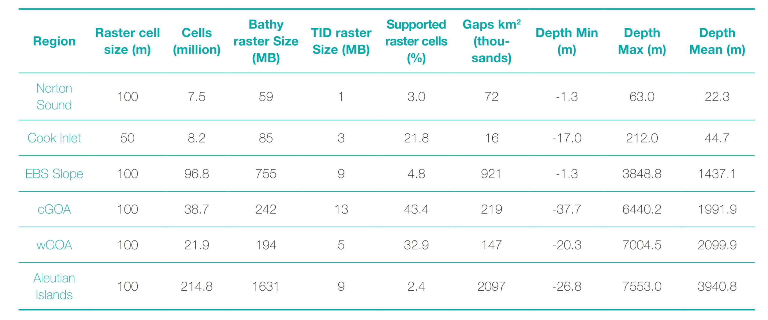
The TID analysis separated the Alaska regional bathymetry rasters by multiple obvious divisions: the large and the small, the well-mapped and the poorly-mapped, and the shallow and the deep (Table 1). Bathymetry rasters ranged in size from 59 MB and 7.5 million cells for Norton Sound to 1,631 MB and 214.8 million cells for the Aleutian Islands (Table 1). As a group, the bathymetry rasters total nearly 3 GB of computer disk storage and nearly 388 million cells. The TIDs were much smaller in size, totaling only 40 MB, roughly a 70-fold decrease in size compared to the bathymetry rasters, and yet still containing the same number of raster cells. The bathymetry rasters of Cook Inlet (21.8 %), the western Gulf of Alaska (32.9 %), and the central Gulf of Alaska (43.4 %) were the most supported by actual depth observations, while those of the Aleutian Islands (2.4 %), Norton Sound (3.0 %), and the eastern Bering Sea Slope (4.8 %) were the least supported. The Norton Sound compilation had the shallowest average depth (x̄ = 22.3 m), Cook Inlet was the next shallowest (x̄ = 44.7 m), and all other rasters averaged > 1,000 m in depth. Minimum depths elevated above MHW in Table 1 are due to cartographic features with high elevations such as prominent rocks or islets.

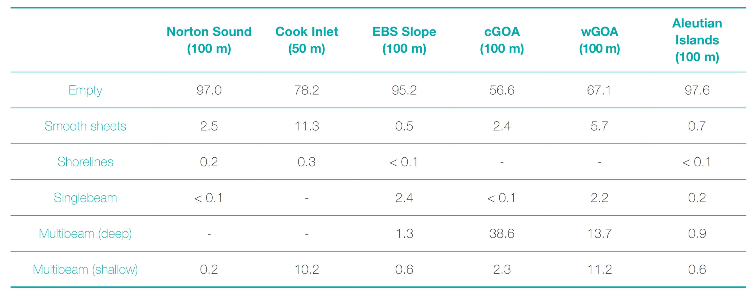
The importance of source data types varied widely among the TIDs (Table 2). Smooth sheet data and its modern equivalent of shallow water multibeam data were the only data classes included in all compilations, with each occupying a maximum of about 11 % of total raster cells in a compilation. Shorelines were digitized for the CI, NS, AI, and EBSS compilations but only accounted for a maximum of 0.3 % of total raster cells, despite totaling nearly 3000 km in length for both the CI (Zimmermann & Prescott, 2014) and NS (Prescott & Zimmermann, 2015) compilations. Singlebeam data were incorporated into all compilations except for CI (Zimmermann & Prescott, 2014), and only a small amount was incorporated into the NS compilation to fill a single gap in Norton Bay (Prescott & Zimmermann, 2015). Large amounts of singlebeam data were incorporated into the WGOA (Zimmermann, et al., 2019b), AI (Zimmermann & Prescott, 2021a), and especially the EBSS compilation (Zimmermann & Prescott, 2018) to cover previously uncharted areas, but the TID analysis showed that these millions of soundings tended to be clumped into few raster cells, limiting their effectiveness at improving maps, and never reaching 3 % occupation of raster cells in any of the compilations. Deep water multibeam was not available for the relatively shallow CI and NS compilations but was important for the WGOA and CGOA compilations, occupying 13.7 % and 38.6 % of raster cells, respectively, the highest data support for this type of bathymetry data among all regional bathymetry compilations.

This analysis of the spatial extent of various data sets collected by numerous platforms also revealed multiple instances of locations that had been mapped more than once. We also located several data sets that would be valuable contributions to our previously published Alaska regional bathymetry rasters but were either unavailable or unknown to us at the time that we compiled the final versions.

5.1 Norton sound

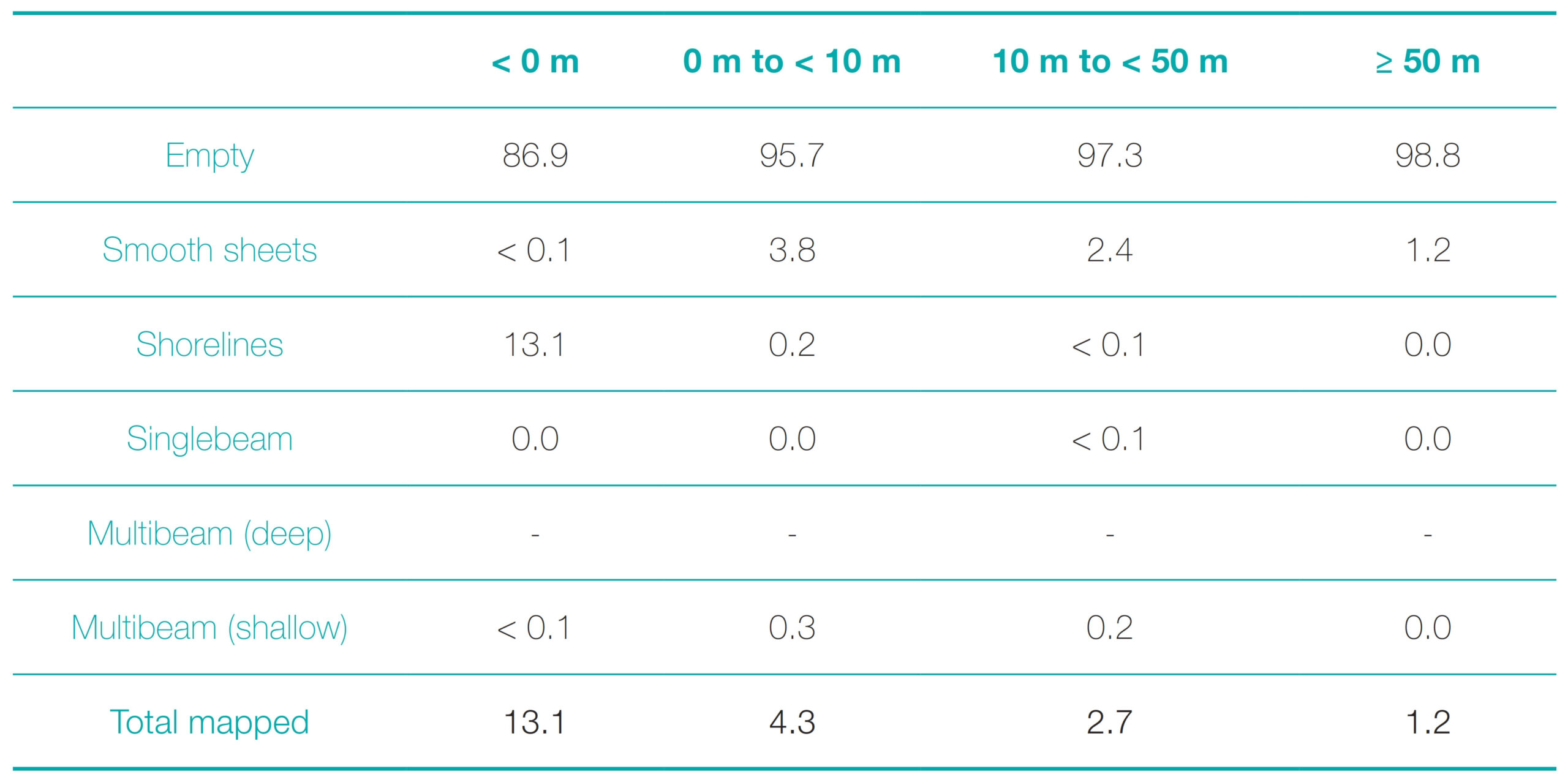
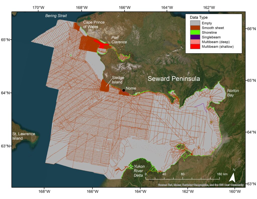
In Norton Sound, the largest unmapped or sparsely mapped areas were north and south of Port Clarence, the eastern half of the sound, off of the Yukon Delta, and along the southern edge of the compilation by St. Lawrence Island. Due to very low contributions from smooth sheet and multibeam data sources, the < 0 m depth zone of NS was sparsely supported with data (13.1 %), mostly from a digitized shoreline (Table 3; Fig. 2). Smooth sheets were the most important data source for the 0 m to < 10 m depth zone but only occupied 3.8 % of cells. Data density decreased rapidly in the 10 m to < 50 m and ≥ 50 m depth zones, with smooth sheets still being the most important data source. The nearly 7,000 singlebeam soundings (Prescott & Zimmermann, 2015) only supported < 0.1 % of raster cells in the 10 m to < 50 m depth zone.

5.2 Cook inlet

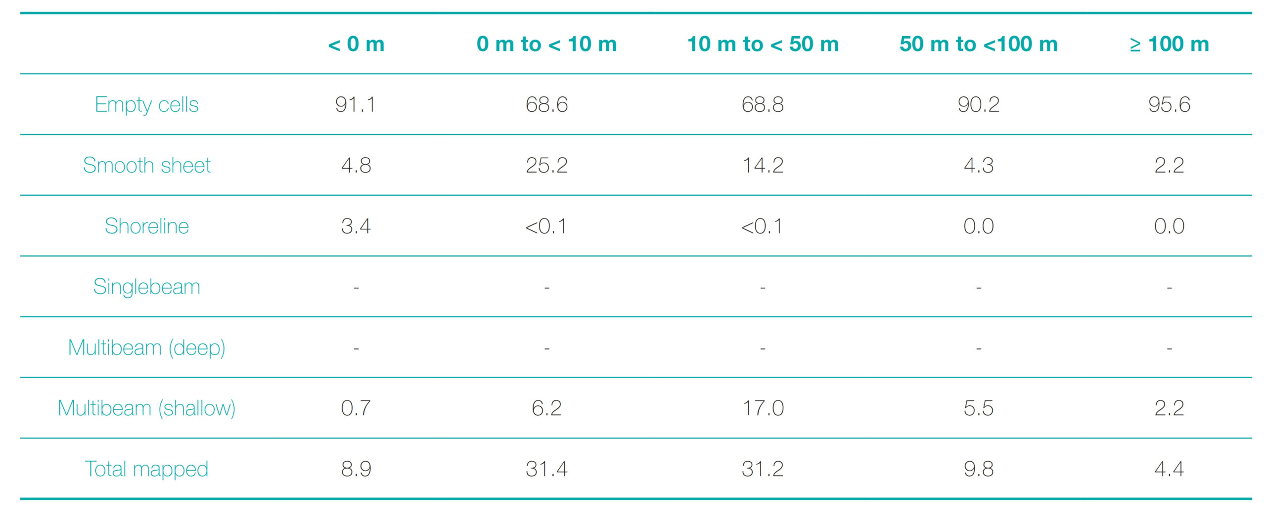
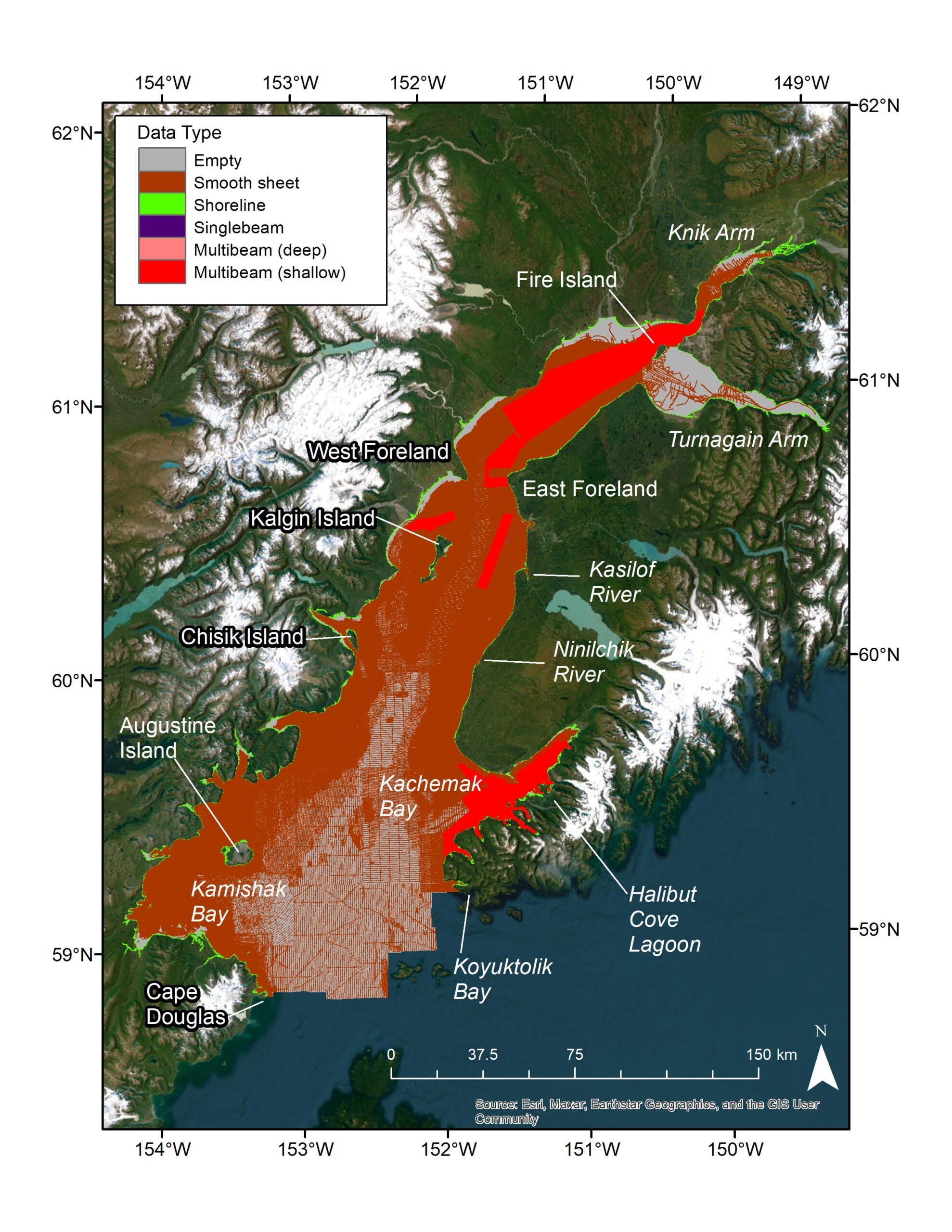
In Cook Inlet, the inshore areas of Turnagain Arm and west of Fire Island were the largest unmapped gaps, while the central, southern area was the sparsest mapped (Fig. 3). Only 8.9 % of the < 0 m depth zone was mapped despite having a digitized shoreline, and these shoreline data were overshadowed by a larger smooth sheet contribution (Table 4). This coverage of the < 0 m depth zone was the lowest among all areas. The 0 m to < 10 m and 10 m to < 50 m depth zones were both 31 % mapped, with the shallower zone more supported by smooth sheet soundings and the deeper zone more supported by multibeam data. There was a sharp decline in occupied cells in the 50 m to < 100 m (9.8 %) and ≥ 100 m (4.4 %) depth zones, both with roughly equal support from smooth sheet and multibeam data sources.

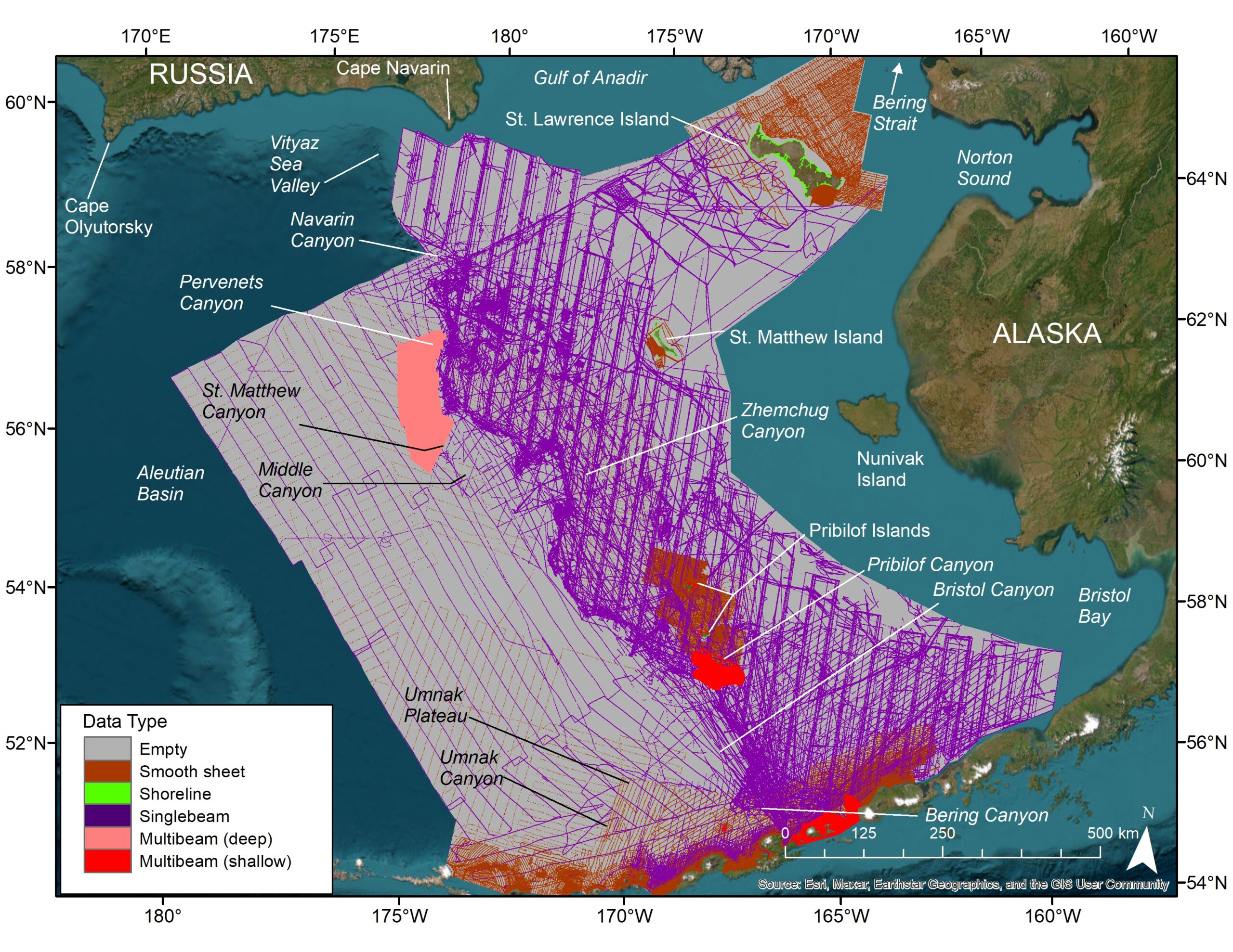
5.3 Eastern Bering Sea slope

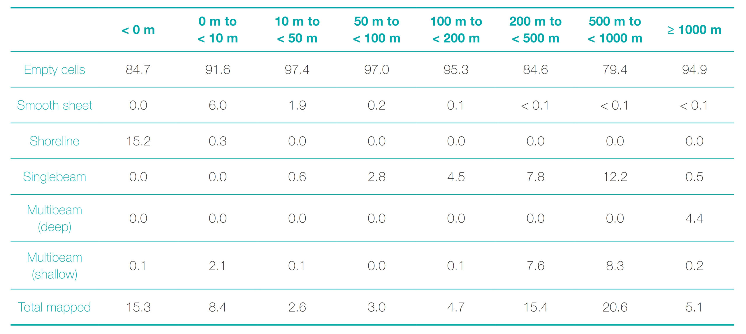
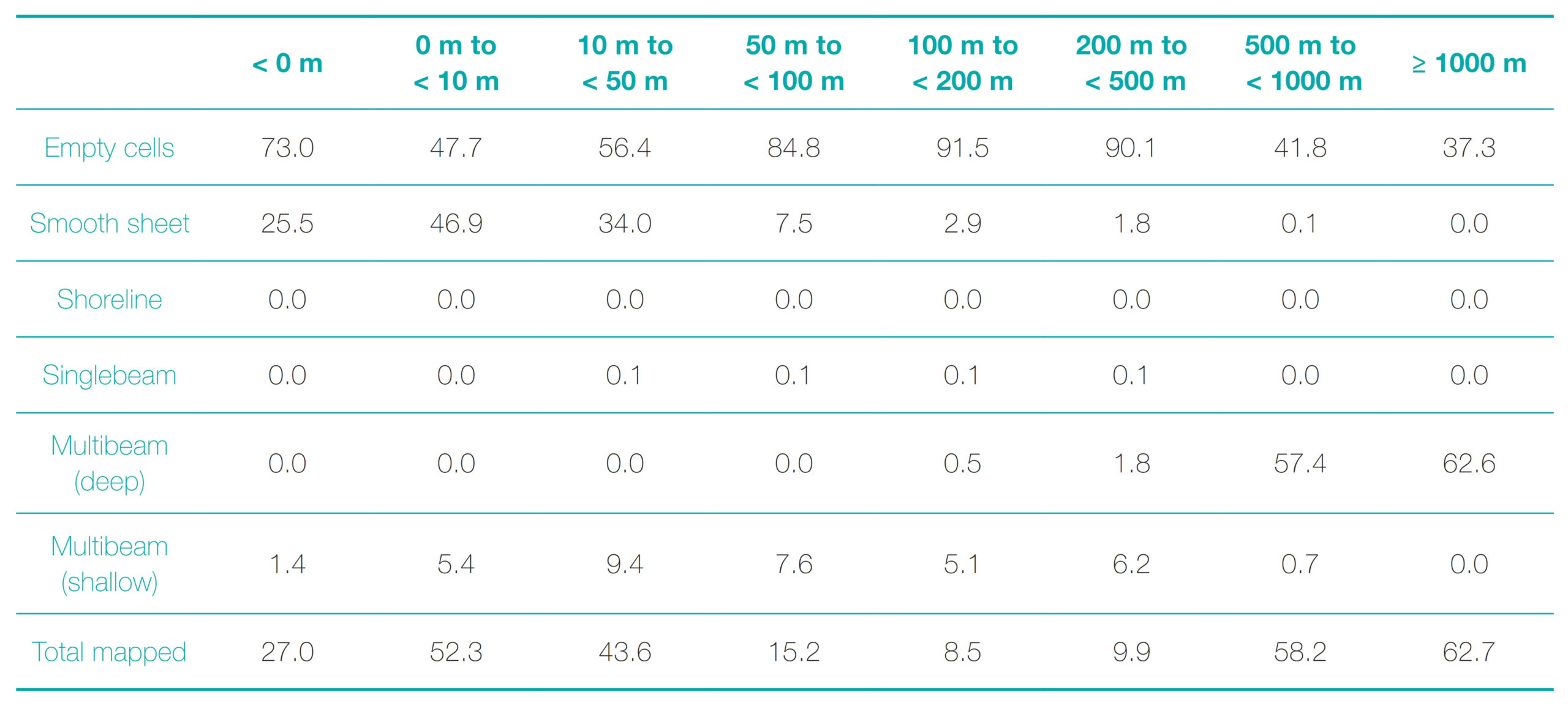
The Aleutian Basin, along with the area between St. Matthew Island, St. Lawrence Island, and the Vityaz Sea Valley, were the most sparsely mapped of the Eastern Bering Sea Slope compilation (Fig. 4). Digitized island shorelines provided nearly all (15.2 % of 15.3 %) of the data in the < 0 m depth zone (Table 5). Data support from all sources decreased by about half in the 0 m to < 10 m depth zone (8.4 %), led by smooth sheets supporting 6.0 % of raster cells, declining to negligible contributions at all deeper depth zones. Data support of all data types further declined to ~ 3 % in the 10 m to < 50 m and 50 m to < 100 m depth zones. Singlebeam data was by far the most important data source in the 100 m to < 200 m depth zone, accounting for nearly all (4.5 % of 4.7 %) data support, and singlebeam supported even higher percentages of raster cells in the 200 m to < 500 m, and 500 m to < 1000 m depth zones, where again it was the most important. Deep water multibeam was the bulk of the data support in the deepest depth zone of ≥ 1,000 m.

5.4 Central Gulf of Alaska

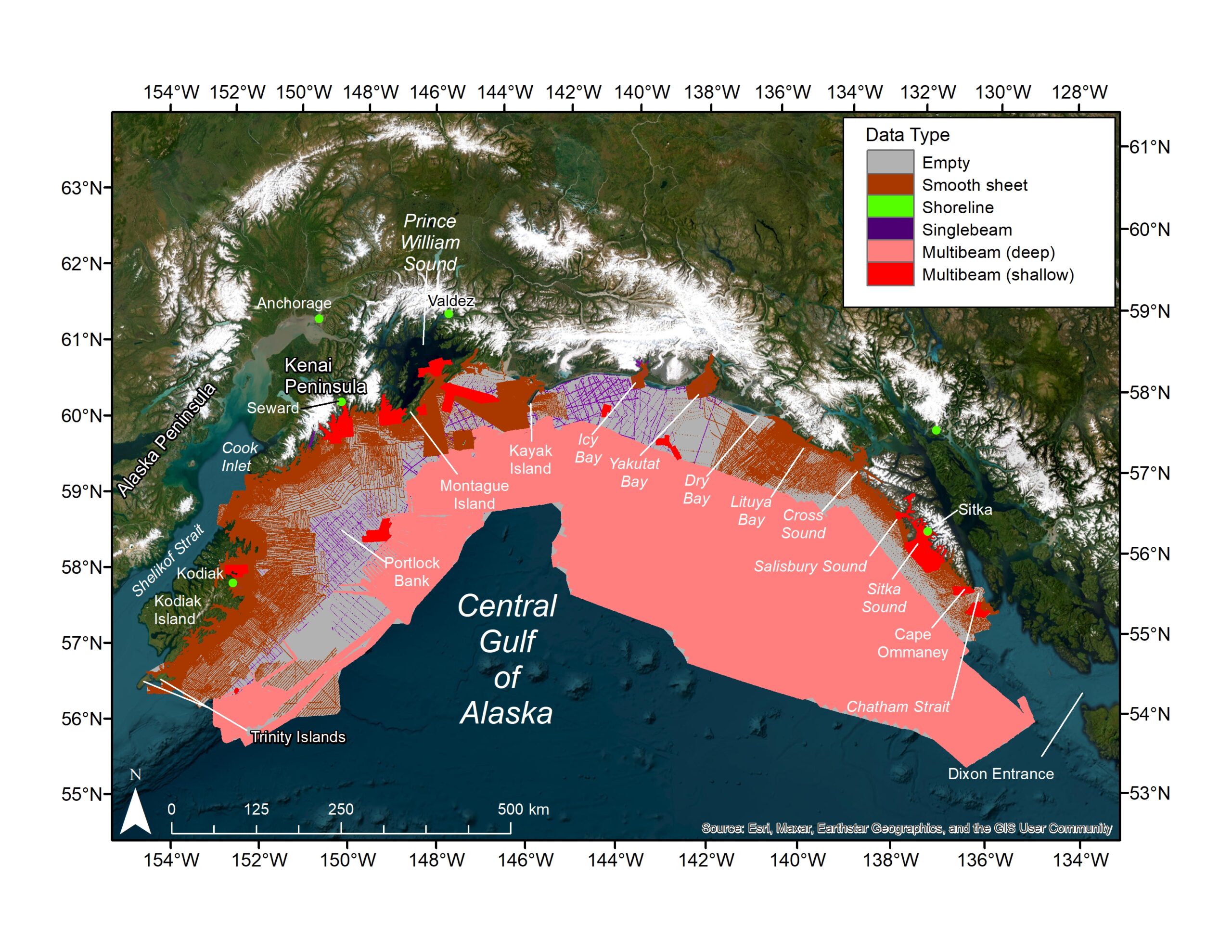
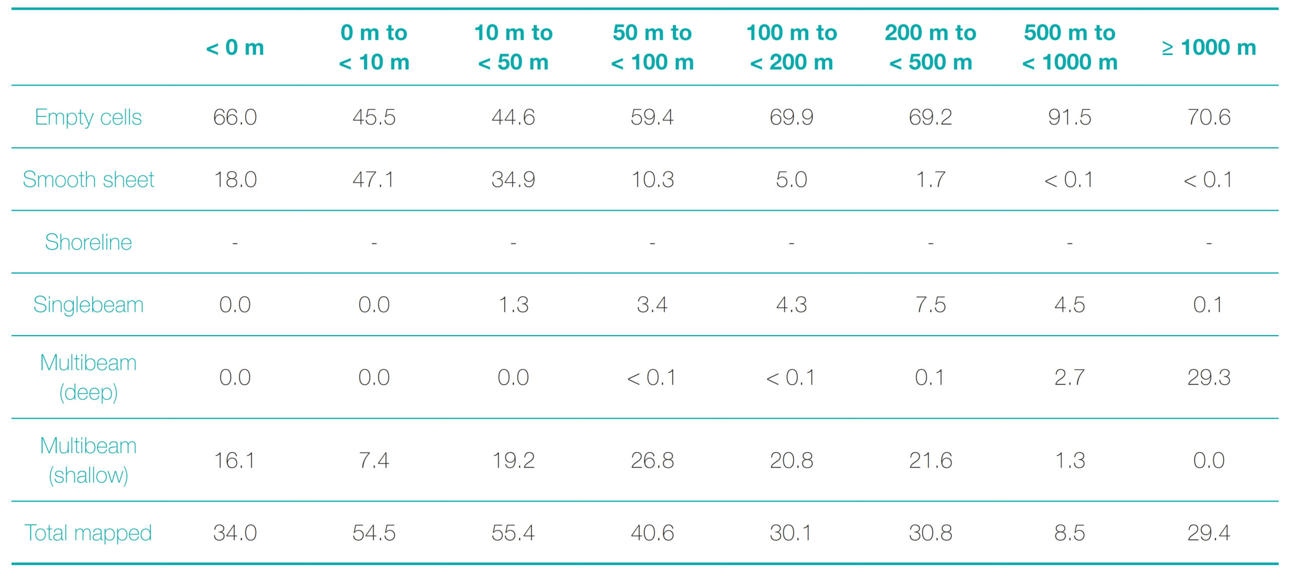
In the Central Gulf of Alaska, the largest unmapped or sparsely mapped gaps occurred on Portlock Bank and south it, south and east of Montague Island, seaward of Yakutat and Icy bays, and shoreward of the deep water multibeam off of Sitka (Fig. 5). Despite the lack of a digitized shoreline, the shallowest depth zone (< 0 m) of the CGOA was well-supported, mainly owing to the contribution of smooth sheet data (25.5 % of 27.0 %), higher than three of the regions (CI, NS, and EBSS) with digitized shorelines (Table 6). Smooth sheet data also provided strong support for the 0 m to < 10 m and 10 m to < 50 m depth zones, making them among the best-supported, similar to that of the AI and WGOA compilations. The 50 m to < 100 m, 100 m to < 200 m, and 200 m to < 500 m depth zones were only moderately supported by smooth sheet and multibeam data and lacked a significant singlebeam contribution, which boosted the support of these depth zones in the AI and WGOA regions. The deepest depth zones of 500 m to < 1000 m and ≥ 1,000 m had the highest data support among all regions (58.2 % and 62.7 %, respectively), mostly due to the deep water multibeam contribution, which helped make the CGOA the most-supported bathymetry raster.

5.5 Western Gulf of Alaska

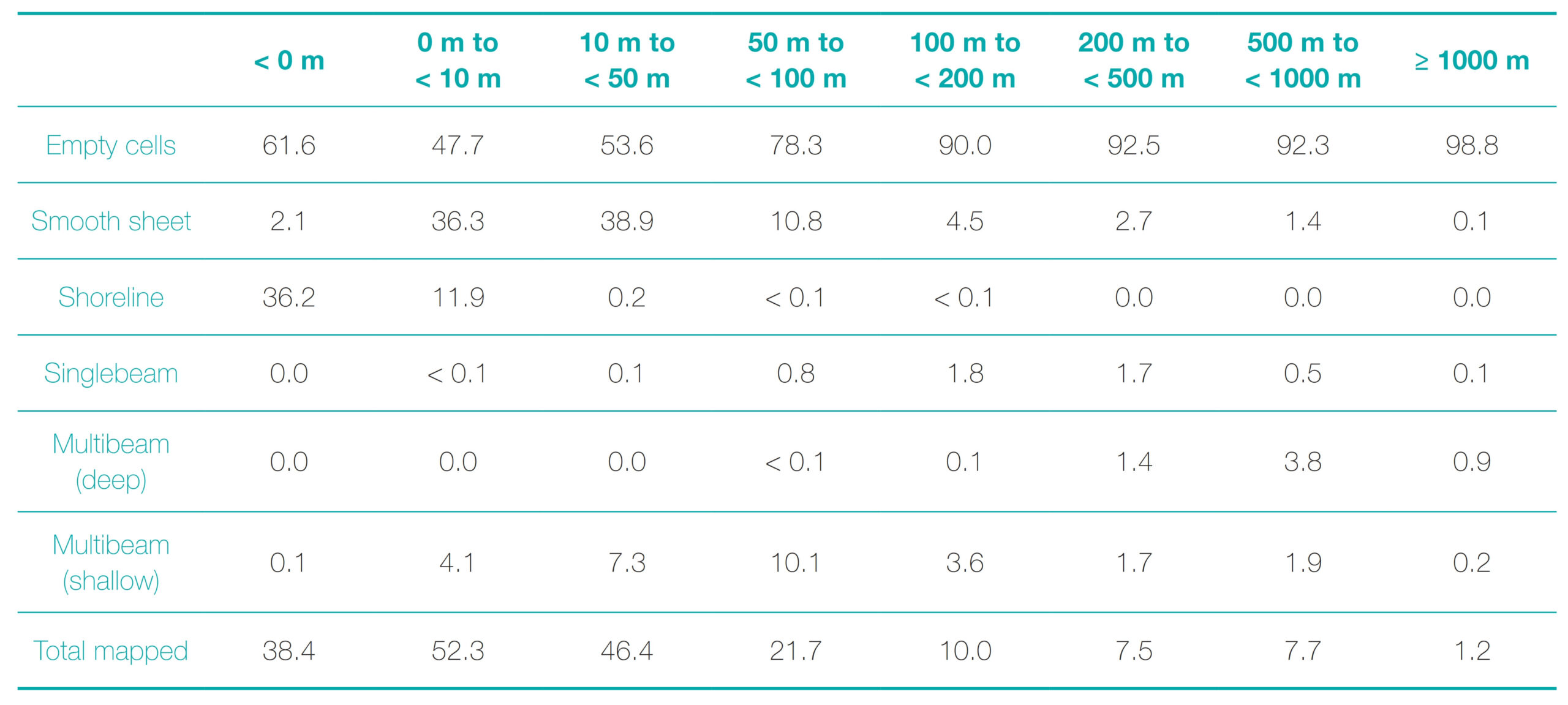
In the Western Gulf of Alaska, the largest unmapped gaps occurred shoreward and seaward of the deep water multibeam along the Aleutian Trench while a small but notable gap occurred in the western Trinity Islands (Fig. 6). Over one-third of the WGOA < 0 m zone was mapped due to nearly equal contributions from smooth sheet and multibeam data sets and without a digitized shoreline (Table 7). The smooth sheet contribution peaked at 47.1 % of available cells in the 0 m to < 10 m depth zone and gradually decreased in deeper depth zones to only 1.7 % at 200 m to < 500 m and to nearly 0 % in the deepest depth zones. Multibeam data was consistently important (~ 20 %) from the 10 m to < 50 m through the 200 m to < 500 m depth zone but declined to only 1.3 % in the 500 m to < 1000 m depth zone and zero in the ≥ 1,000 m depth zone. The singlebeam contribution was greater in deeper water, gradually increasing from 1.3 % in the 10 m to < 50 m zone and peaking at 7.5 % in the 200 m to < 500 m zone before declining to 0.1 % in the deepest waters. Deep water multibeam accounted for nearly all of the 29.4 % of occupied cells in the ≥ 1000 m depth zone, and this support greatly increased the overall data occupancy for the WGOA compilation.

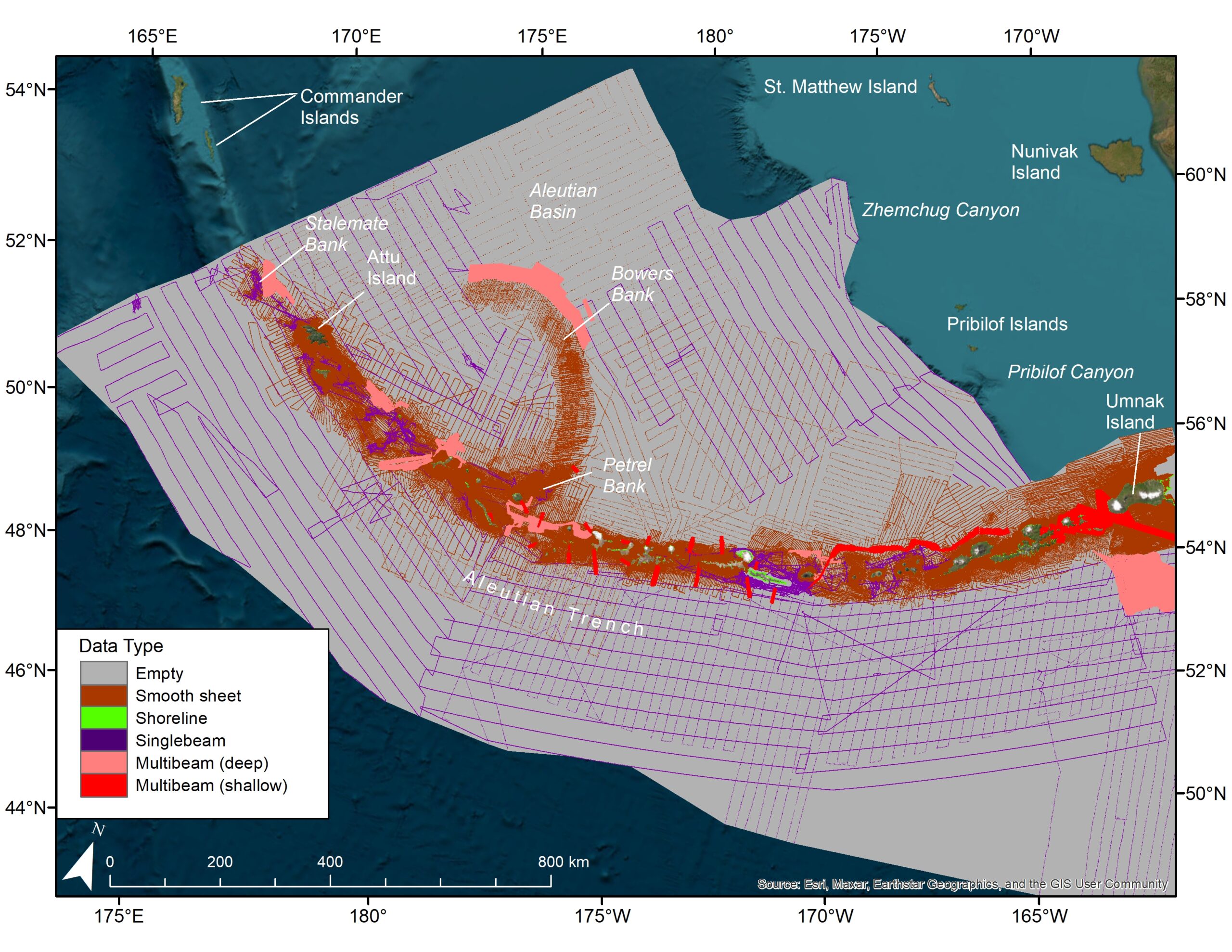
5.6 Aleutian Islands

In the Aleutian Islands, bathymetry gaps occurred essentially everywhere except in a narrow 200 km wide band along the islands and on Petrel, Bowers, and Stalemate banks (Fig. 7). The digitized shoreline in the AI provided the highest support of the < 0 m and 0 m to < 10 m depth zones among all bathymetry raster compilations (Table 8). About 50 % of raster cells were supported in both the 0 m to < 10 m and 10 m to < 50 m depth zones, mostly on the contribution of smooth sheets. Smooth sheets and multibeam data equally supported the 50 m to < 100 m depth zone, together accounting for 20.9 % of raster cells, more than in all other compilations except the WGOA. The depth zones of 100 m to < 200 m, 200 m to < 500 m, and 500 m to < 1,000 m were moderately supported (7.5 % to 10.0 %) by a mixture of low amounts of smooth sheet, singlebeam, multibeam and deep water multibeam. None of the data types, including deep water multibeam, supported even 1 % of the deepest depth zone of ≥ 1,000 m, making it the least-supported deep zone among all compilations.

5.7 Overlap or Double-mapping

The purpose of creating the TIDs is both to help identify areas needing new mapping efforts and areas that have been previously well-mapped. During this analysis, we became aware of multiple instances of double-mapping in Alaska waters. Here we describe these examples and how they might have been avoided with better guidance about what has and has not been mapped.

5.7.1 Chirikof Island overlap

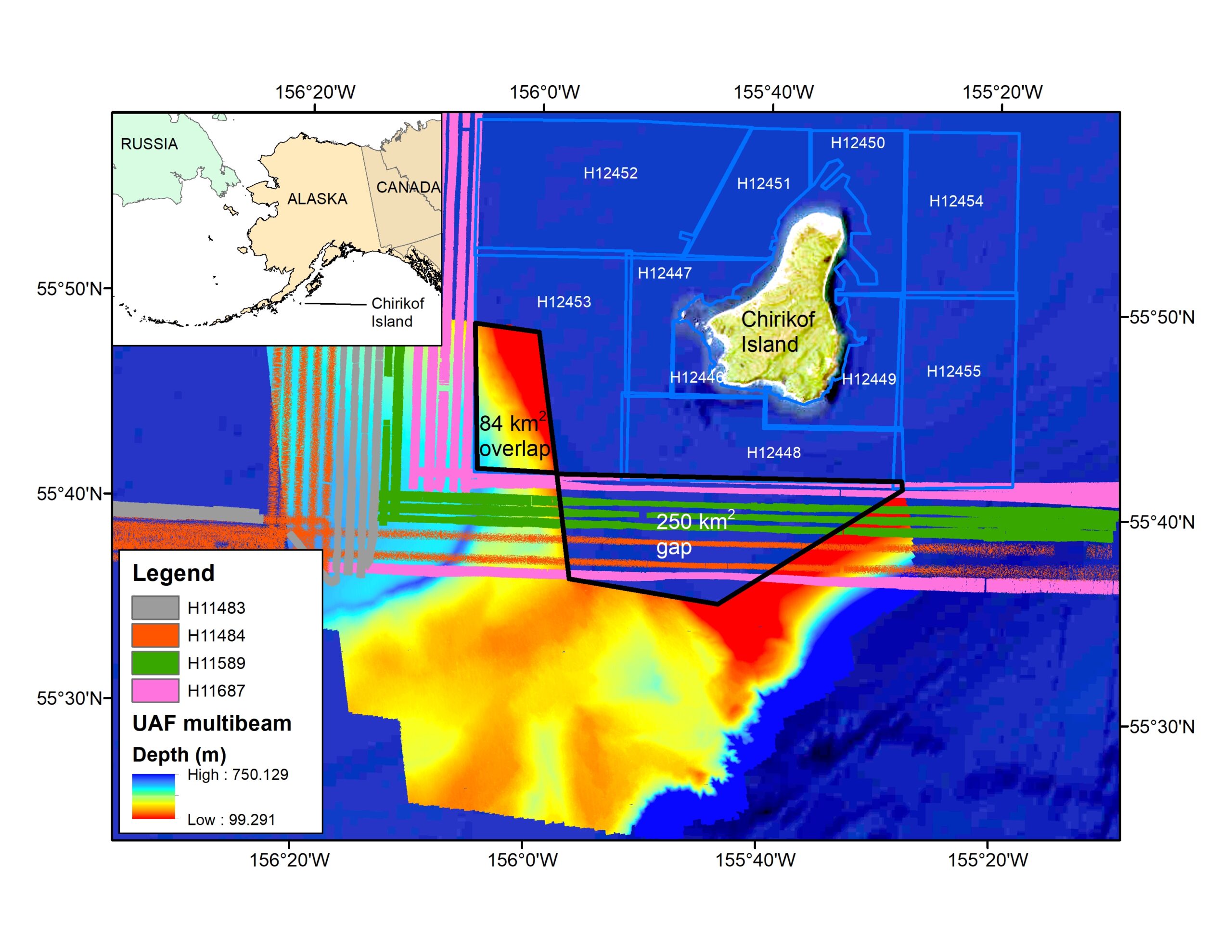
The University of Alaska Fairbanks (UAF) hired Thales GeoSolutions in 2001 to map with multibeam an area of about 1,600 km2 (hydrographic survey W00267) with a 10 m horizontal resolution raster, 10 km to 20 km southwest of Chirikof Island, for geomorphological analysis of fish and invertebrate habitats (Fig. 8). Apparently, without knowledge of this 2001 multibeam effort, NOS made multiple, coarse, widely spaced multibeam transects across the north portion of this Thales GeoSolutions multibeam at resolutions of 25 m (H11483, 2005), 5 m (H11484: 2005 reconnaissance, partial coverage), 20 m (H11589, 2006), and 16 m (H11687, 2007). These generally coarse survey transects followed the cardinal directions, meeting at right angles. In 2012, NOS returned and conducted 10 multibeam surveys forming a rectangle around Chirikof Island, adjoining one of the right-angled junctions of the earlier coarse survey transects, presumably to avoid overlap and provide continuity with the older surveys. All of these 2012 surveys had horizontal resolutions < 10 m except for surveys in the SE (H12455) and SW (H12453) corners of the rectangle that were completed at a resolution of 16 m. The SW corner of the SW survey overlapped the Thales GeoSolutions survey by about 84 km2 but left a gap of approximately 250 km2 between the southern edge of H12453, its neighbor H12488 and the UAF/Thales Geo-Solutions map. This 250 km2 gap was partially covered by some of the coarse transects but inadequately mapped. Overall it would have been beneficial to coordinate these various mapping activities such that a homogenous, 10 m horizontal resolution multibeam map of the shallower waters surrounding Chirikof Island could be constructed.

5.7.2 Kodiak Island overlap

In 2012, the Alaska Department of Fish and Game (ADFG) mapped two areas at a horizontal resolution of 10 m for crab habitat research (Fig. 9) in Marmot and Chiniak bays near Kodiak Island (each roughly 100 km2 in size)¹⁶. They used a relatively inexpensive entry-level WASSP (Wide Angle Sonar Seafloor Pro-filer) multibeam that can be installed on fishing boats and integrated with navigational software such as Nobeltec’s TimeZero¹⁷. NOS had already mapped the southern portion of Marmot Bay with multibeam in 2011 and completed the northern portion in 2012. NOS had also mapped with multibeam the central portion of Chiniak Bay in 1999 (H10913, 10 m) and completed the remainder in 2017. Thus, about 200 km2 of seafloor was double-mapped.

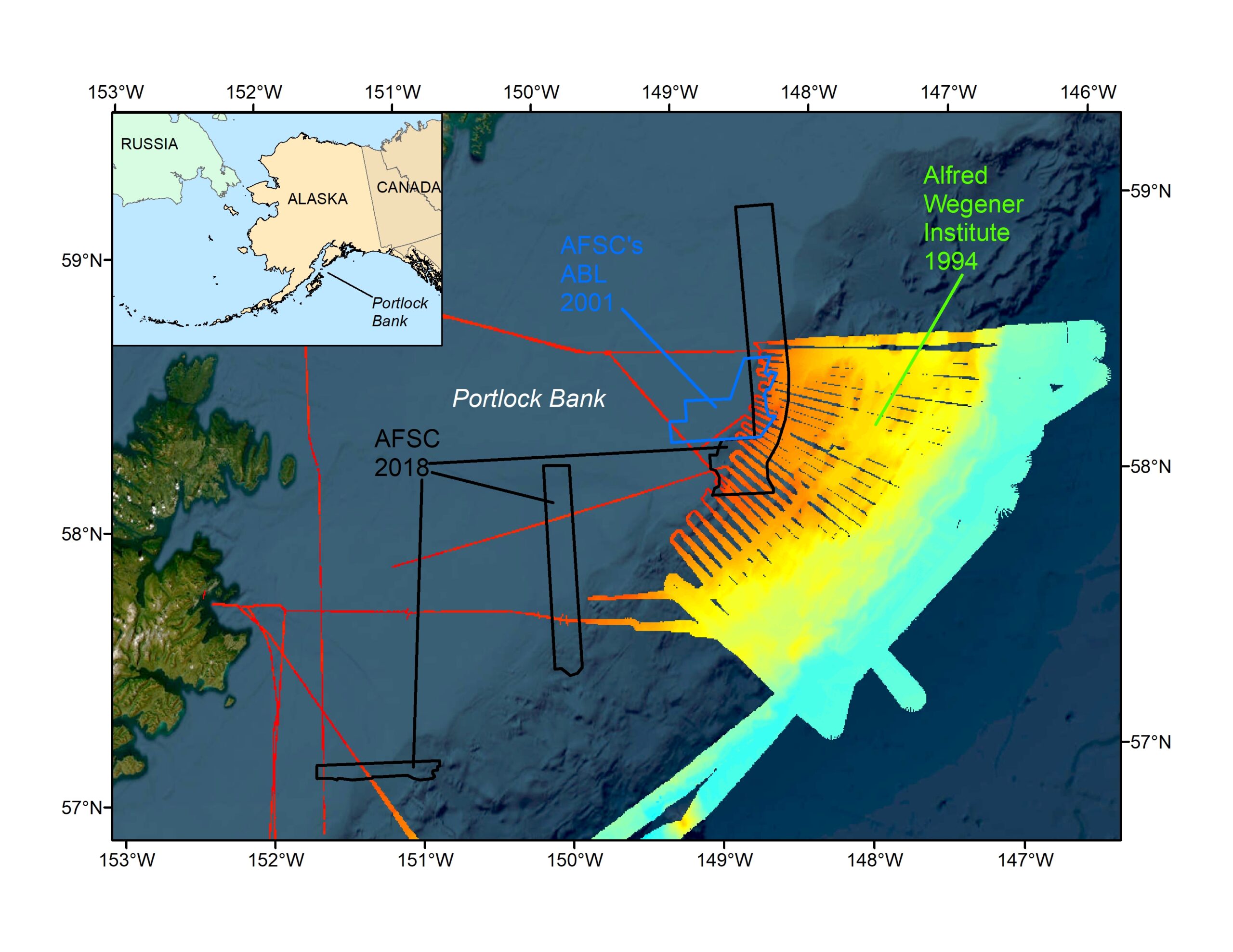
5.7.3 Portlock Bank overlap

Multiple cruises mapped with multibeam the eastern edge of Portlock Bank in recent years (Fig. 10). The first and second cruises for plate tectonics research occurred on the R/V Sonne in 1994 (SO-96-2¹⁸, and SO-97-1¹⁹), utilized a deep water multibeam, and followed a fan-like survey pattern, where there were overlaps between transects in deeper water (~ > 2,000 m) but gaps between transects in the shallower waters (~ 200 m) of eastern Portlock Bank. This partial mapping covered about 15,000 km2. The AFSC’s Auke Bay Laboratories hired Thales GeoSolutions’s R/V Davidson to map with multibeam about 790 km2 of eastern Portlock Bank in 2001 for describing fish and invertebrate habitats (Rooney, 2008), with deeper portions of their survey (to about 740 m) overlapping with the shallower portion of the R/V Sonne surveys. In 2018, the Seattle office of the AFSC chartered the NOAA ship Fairweather to map several portions of the central Gulf of Alaska with multibeam for fish habitat analysis, and their easternmost area overlapped by about 500 km2 with the R/V Sonne 1994 and by about 200 km2 with the Davidson 2001 areas, with some areas being triple-mapped. Thus, some knowledge of the previous mapping and research interests among geologists and fish biologists at eastern Portlock Bank could have benefitted all parties. The top of Portlock Bank remains one of the noteworthy, shallow, unmapped areas in the Gulf of Alaska (Zimmermann & Prescott, 2015).

6 Discussion

The TID analysis revealed new information about the Alaska regional bathymetry rasters, highlighting areas within each bathymetry raster of high-quality data and depicting areas with low-quality or no data. For example, vast, deep (> 1000 m) areas within the AI compilation are almost completely unmapped. Some entire rasters could use a great deal of improvement, such as NS, while other rasters, such as CI, are relatively well-mapped. Efforts to complete a bathymetry map of the Alaska EEZ in support of the Seabed 2030 project may focus on either upgrading the published rasters by adding more soundings of higher quality data types or by conducting new mapping expeditions in gap areas. The TID raster files are substantially smaller than the bathymetry rasters and, therefore, should be more easily utilized.

6.1 Effort spent on different data types

Each Alaska regional bathymetry compilation takes a finite amount of time and resources, with more emphasis placed on processing data sets judged likely to create a good map. For example, we would prefer a new, large-scale, and fully digital multibeam survey, which would take minutes of processing time, rather than to digitize an older, small-scale smooth sheet, which would take days of processing time. Despite our best efforts to triage data sets, sometimes beneficial data sets do not get examined or incorporated, and detrimental or difficult to process data sets get included when they should not have been. Digitizing the thousands of kilometers of shoreline for the CGOA and WGOA compilations would have improved the coverage of this shallowest depth category but at a very significant effort for shallow (< 0 m) areas that were already relatively well-mapped (Table 6; 27.0 % and Table 7; 34.0 %, respectively). Digitizing the shoreline for NS, AI, and the EBSS paid off well, significantly improving coverage of the < 0 m depth zone, but was much less helpful for CI, an outcome that we interpret to be due to extensive mud flats occurring between the shoreline and shallowest soundings. Smooth sheet data density in CI was deemed sufficient for constructing the bathymetry raster without the addition of available non-hydrographic singlebeam data sets, which might have added more errors than useful soundings to help define the seafloor. The generally high levels of sounding coverage in CI depth zones < 50 m verified the merit of this approach but depth zones > 100 m may have benefitted from the additional soundings. The sparse coverage of all depth zones > 0 m in NS and the 100 m to < 200 m and 200 m to < 500 m depth zones of COA may have benefitted from additional singlebeam data above the small amounts already incorporated. While highly beneficial in some regional compilations, the clumped nature of the singlebeam data limited its impact, and it is still not clear if it is preferable to go through the slower process of selecting the seafloor from the higher density raw echosounder data or to utilize the unproofed but sparser, more distributed data from a navigation file. The unproofed navigation file data undoubtedly introduced seafloor feature errors in some areas but time lost to the laborious raw echosounder file editing meant no data could be processed for other unmapped areas.

6.2 Additional bathymetry data sets

New data sets are continually emerging during or immediately after the final raster version is completed. While these new data would have improved the compilations, adding them would have delayed publication. For example, multibeam survey H13035 (2017) of the previously unmapped Coal Bay (see Figs. 1 and 2 in Zimmermann et al., 2019b) was made publicly available when the WGOA bathymetry raster was being finalized and published.

Other significant data sets not in the TIDs include regions of new NOS multibeam in the WGOA, in the Port Clarence area of NS, and around Kodiak Island in the CGOA. There are also seven additional maps of older deep water back-arc areas in the AI²⁰, beyond the eight that were included in the most recent edition of the AI bathymetry raster (Zimmermann & Prescott, 2021a), available from the University of South Carolina. Caladan Oceanic²¹ mapped 72,000 km2 of the deepest portion of the Aleutian Trench in 2020, following their global 2018–2019 Five Deeps Expedition (Bongiovanni, 2022), where the AI raster only had sparse soundings approximating this area (Fig. 7). Numerous unprocessed singlebeam and navigational files are available from newer bottom trawl cruises in the Gulf of Alaska which might improve coverage in the CGOA raster, especially in the relatively unmapped shelf area off of Icy and Yakutat bays (Fig. 5; also see Fig. 4 from Zimmermann & Prescott, 2015).

6.3 Additional bathymetry data sources

Some international data sources, such as the Japan Agency for Marine-Earth Science and Technology (JAMSTEC) and the Korea Polar Research Institute (KOPRI), were not known to us and, therefore, not included in any of the Alaska regional bathymetry compilations, while additional data are available from the Alfred Wegener Institute (AWI), Helmholtz Centre for Polar and Marine Research beyond that already included in the CGOA and WGOA compilations. Bathymetry data from the commercial fishing industry are generally regarded as proprietary rather than public property because the detailed compilations of specific locations can reveal preferred fishing areas and breaches of areas that are closed to fishing or transit, such as the Steller sea lion (Eumetopias jubatus) rookeries²². If large volumes of high-quality bathymetry data can be collected during fishing operations, such as with the WASSP multibeam utilized by ADFG near Kodiak Island, without the standard corrections and calibrations that are routinely conducted during hydrographic multibeam surveys (e.g., speed-of-sound, patch test, bar checks, etc.), then this approach may result in the democratization of seafloor mapping. Fishing industry data remain a tremendous, mostly untapped resource (a small amount was incorporated only in the EBSS compilation; Zimmermann & Prescott, 2018). In 2018, NOAA announced²³ the hosting of a Crowdsourced Bathymetry (CSB) database, developed in coordination with the International Hydrographic Organization’s (IHO) CSB Working Group as a formal means of capturing domestic and international non-hydrographic data sources, that are not intended to be used for navigational purposes but might be perfectly suitable to the Seabed 2030 project. Hopefully, all of the Alaska regional bathymetry rasters can be updated with new data and combined into a complete map fully covering the Alaska EEZ in the future.

6.4 Dates of bathymetry collection

It is expected that depth and navigational data quality generally should improve over time, with newer hydrographic surveys superseding older surveys. We incorporated this trend in technological advancement in our Alaska regional bathymetry compilations by removing the overlap of older, lower-quality surveys where newer, higher-quality surveys were available, as indicated by our ranking of data types (e.g., multibeam supersedes smooth sheet). Otherwise, we included all available bathymetry data, regardless of collection date, with the CI (Zimmermann & Prescott, 2014), CGOA (Zimmermann & Prescott, 2015), NS (Prescott & Zimmermann, 2015), and WGOA (Zimmermann et al., 2019b) bathymetry rasters incorporating sources over a century in age. Once new data are available, overlaps of the older, lower quality data are removed, a new TIN is created and then converted into an updated bathymetry raster (Zimmermann & Prescott, 2021a). Other summaries of mapped areas have limited their analyses to more recent data (e.g., collected since 1960: Westington et al., 2018a, 2018b), which removes much of the coverage of Alaska. Since previous analyses show that Gulf of Alaska hydrographic surveys dating as far back as the 1930s have low mean discrepancies (-2.6 % to 3.4 %) compared to depths derived from recent acoustics (Zimmermann et al., 2019a), we chose to maintain this inclusive approach. Also, the methods of constructing these Alaska regional bathymetry compilations included proofing the digital soundings hosted at NCEI against the source document – the correctly georeferenced smooth sheet and shifting soundings hundreds or thousands of meters so that they plot in the correct place (Zimmermann & Benson, 2013). This extra step is critical for making sense of these older data sets, as this also allows for correction of misdigitized soundings or features, deletion of repeated soundings, and digitization of missing soundings. It is important to consider that many of these older soundings were the foundation of the earliest navigational charts and until newer surveys are conducted, these older soundings remain on the charts and are routinely used by mariners.

6.5 Cook Inlet raster resolution

Assembling the high-quality and high-density bathymetric data in the Cook Inlet region provided a stark contrast to assembling bathymetry data in poorly mapped areas in Alaska (Zimmermann & Prescott, 2014). Most of these CI surveys were conducted recently (since the mid-1960s), in the relatively modern horizontal datum of NAD27 (North American Datum of 1927), and at large scales, as a response to the unprecedented seafloor changes caused by the Great Earthquake of 1964 (Zimmermann & Prescott, 2014). Therefore, it was decided to increase the horizontal resolution of the bathymetry raster from the somewhat arbitrary and coarse 100 m used in all the other Alaska regional bathymetry compilations to 50 m, a four-fold change in data density, without a formal analysis. The TID analyses examined in this project demonstrate that data support of the 50 m Cook Inlet raster compares favorably to the other 100 m rasters and that the decision to increase the resolution was well-justified.

6.6 Double-mapping

Any duplication of mapping effort, such as the three examples we described in this analysis, is an unfortunate and avoidable occurrence. Greater communication should prevent future instances from happening. Unfortunately sometimes double-mapping is planned on purpose, such as the Saildrone deep water multibeam targeting the Ingenstrem and Buldir depressions in the summer of 2022, areas previously mapped in 2005 (Coombs et al., 2007). When double-mapping does occur, it can provide an opportunity to quantify changes in depth and to identify the processes responsible (e.g., Zimmermann et al., 2018; Zimmermann et al., 2022)

7 Conclusion

The path forward to completing the seafloor map of the Alaska EEZ, and supporting the global Seabed2030 effort, is to make the most judicious use of our limited at-sea resources. Here we provide smallsized TIDs for use as guides for sounding the unmapped gaps that we identified. We expect that formal mapping efforts by hydrographic-quality cruises will continue to supply important, definitive data sets but only in very limited areas. The funding for dedicated mapping cruises is relatively small and there are too few vessels conducting this work. To achieve Seabed2030’s goals we need to harness the effort of the more common non-hydrographic research cruises, and the more numerous fishing vessels, already operating in remote and often poorly mapped areas. A shared and more authoritative seafloor map should improve the management of our natural resources, upgrade oceanographic and climate modeling efforts, and inform our ocean policies

Acknowledgements

Thanks to Map the Gaps organization for inspiration and allowing us to use their name. Thanks to Lukas DePhilippo, Nazila Merati, Ned Laman, Michael Martin, and two anonymous reviewers for constructive reviews. Thanks to GEBCO (the General Bathymetric Chart of the Oceans) and The Nippon Foundation – GEBCO Seabed 2030 Project. Thanks to the staff at NCEI (National Centers for Environmental Information²⁴) for frequent assistance with smooth sheets. The findings and conclusions in the paper are those of the authors and do not necessarily represent the views of the National Marine Fisheries Service. Any use of trade, product, or firm names in this publication is for descriptive purposes only and does not imply endorsement by the U.S. Government.

References

Bongiovanni, C., Stewart, H. A. and Jamieson, A. J. (2022). High‐resolution multibeam sonar bathymetry of the deepest place in each ocean. Geosci. Data J., 9, 108–123. http://doi. org/10.1002/gdj3.122

Coombs, M. L., White, S. M. and Scholl, D. W. (2007). Massive edifice failure at Aleutian arc volcanoes. Earth and Planetary Science Letters, 256(3-4), 403–418.

GEBCO Bathymetric Compilation Group 2022 (2022). The GEBCO_2022 Grid a continuous terrain model of the global oceans and land. NERC EDS British Oceanographic Data Centre NOC. doi:10.5285/e0f0bb80-ab44-2739-e053-6c86abc0289c

Hoff, G. R. (2016). Results of the 2016 eastern Bering Sea upper continental slope survey of groundfish and invertebrate resources. U.S. Dep. Commer., NOAA Tech. Memo. NMFSAFSC-339, 272 p.

Jakobsson, M., Mayer, L. A., Bringensparr, C., Castro, C. F., Mohammad, R., Johnson, P. et al. (2020). The international bathymetric chart of the Arctic Ocean version 4.0. Scientific Data, 7(1), 1–14.

Laman, E. A., Rooper, C. N., Rooney, S. C., Turner, K. A., Cooper, D. W. and Zimmermann, M. (2017). Model-based essential fish habitat definitions for Bering Sea groundfish species. U.S. Dep. Commer., NOAA Tech. Memo. NMFS-AFSC-357, 265 p.

Lauth, R. R., Dawson, E. J. and Conner, J. (2019). Results of the 2017 eastern and northern Bering Sea continental shelf bottom trawl survey of groundfish and invertebrate fauna. U.S. Dep. Commer., NOAA Tech. Memo. NMFS-AFSC-396, 260 p.

Mayer, L., Jakobsson, M., Allen, G., Dorschel, B., Falconer, R., Ferrini, V., Lamarche, G., Snaith, H. and Weatherall, P. (2018). The Nippon Foundation—GEBCO seabed 2030 project: The quest to see the world’s oceans completely mapped by 2030. Geosciences, 8(2), 63.

Prescott, M. M. and Zimmermann, M. (2015). Smooth sheet bathymetry of Norton Sound. U.S. Dep. Commer., NOAA Tech. Memo. NMFS-AFSC-298, 23 p.

Rooney, S. C. (2008). Habitat analysis of major fishing grounds on the continental shelf off Kodiak, Alaska. Doctoral dissertation, University of Alaska Fairbanks.

Rooney, S., Rooper, C. N., Laman, E. A., Turner, K., Cooper, D. and Zimmermann, M. (2018). Model-based Essential Fish Habitat definitions for Gulf of Alaska groundfish species. U.S. Dep. Commer., NOAA Tech. Memo. NMFS-AFSC-373, 370 p.

Sigler, M. F., Rooper, C. N., Hoff, G. R., Stone, R. P., McConnaughey, R. A. and Wilderbuer, T. K. (2015). Faunal features of submarine canyons on the eastern Bering Sea slope. Marine Ecology Progress Series, 526, 21–40.

Turner, K., Rooper, C. N., Laman, E. A., Rooney, S. C., Cooper, D. W. and Zimmermann, M. (2017). Model-based essential fish habitat definitions for Aleutian Island groundfish species. U.S. Dep. Commer., NOAA Tech. Memo. NMFS-AFSC-360, 239 p.

von Szalay, P. G. and Raring, N. W. (2016). Data report: 2015 Gulf of Alaska bottom trawl survey. U.S. Dep. Commer., NOAA Tech. Memo. NMFS-AFSC-325, 249 p.

von Szalay, P. G. and Raring, N. W. (2020). Data Report: 2018 Aleutian Islands bottom trawl survey. U.S. Dep. Commer., NOAA Tech. Memo. NMFS-AFSC-409, 175 p.

Weatherall, P., Marks, K. M., Jakobsson, M., Schmitt, T., Tani, S., Arndt, J. E., Rovere, M., Chayes, D., Ferrini, V. and Wigley, R. (2015). A new digital bathymetric model of the world’s oceans. Earth and Space Science, 2(8), 331–345.

Westington, M., Varner, J., Johnson, P., Sutherland, M., Armstrong, A. and Jencks, J. (2018a). Assessing Sounding Density for a Seabed 2030 Initiative. Proceedings of the Canadian Hydrographic Association, 20 pp.

Westington, M., Varner, J., Johnson, P., Sutherland, M., Armstrong, A. and Jencks, J. (2018b). Assessing Gaps via Bathymetric Sounding Density. The International Hydrographic Review, 20, 41–43.

Zimmermann, M. and Benson, J. L. (2013). Smooth sheets: How to work with them in a GIS to derive bathymetry, features and substrates. U.S. Dep. Commer., NOAA Tech. Memo. NMFSAFSC-249, 52 p.

Zimmermann, M. and Prescott, M. M. and Rooper, C. N. (2013). Smooth sheet bathymetry of the Aleutian Islands. U.S. Dep. Commer., NOAA Tech. Memo. NMFS-AFSC-250, 43 p.

Zimmermann, M. and Prescott, M. M. (2014). Smooth sheet bathymetry of Cook Inlet, Alaska. U.S. Dep. Commer., NOAA Tech. Memo. NMFS-AFSC-275, 32 p.

Zimmermann, M. and Prescott, M. M. (2015). Smooth sheet bathymetry of the central Gulf of Alaska. U.S. Dep. Commer., NOAA Tech. Memo. NMFS-AFSC-287, 54 p.

Zimmermann, M. and Prescott, M. M. (2018). Bathymetry and Canyons of the Eastern Bering Sea Slope. Geosciences: Special Issue Marine Geomorphometry, 8(5), 184. https://doi. org/10.3390/geosciences8050184

Zimmermann, M., Ruggerone, G. T., Freymueller, J. T., Kinsman, N., Ward, D.H. and Hogrefe, K. (2018). Volcanic ash deposition, eelgrass beds, and inshore habitat loss from the 1920s to the 1990s at Chignik, Alaska. Estuarine, Coastal and Shelf Science. 202, 69–86. https://doi.org/10.1016/j.ecss.2017.12.001

Zimmermann, M., De Robertis, A. and Ormseth, O. (2019a). Verification of historical smooth sheet bathymetry. Deep Sea Research Part II: Topical Studies in Oceanography: Understanding Ecosystem Processes in the Gulf of Alaska, 2(165), 292–302. https://doi.org/10.1016/j.dsr2.2018.06.006

Zimmermann, M., Prescott, M. M and Haeussler, P. J. (2019b). Bathymetry and Geomorphology of Shelikof Strait and the Western Gulf of Alaska. Geosciences: Special Issue Geological Seafloor Mapping, 9(10), 409. https://doi.org/10.3390/geosciences9100409

Zimmermann, M. and Prescott, M. M. (2021a). Passes of the Aleutian Islands: First detailed description. Fisheries Oceanography, 30(3), 280–299. http://dx.doi.org/10.1111/fog.12519

Zimmermann, M. and Prescott, M. M. (2021b). False Pass, Alaska: Significant changes in depth and shoreline in the historic time period. Fisheries Oceanography, 30(3), 264–279. http://dx.doi. org/10.1111/fog.12517

Zimmermann, M., Erikson, L. H., Gibbs, A. E., Prescott, M. M., Escarzaga, S. M., Tweedie, C. E., Kasper, J. L. and Duvoy, P.X. (2022). Nearshore bathymetric changes along the Alaska Beaufort Sea coast and possible physical drivers. Cont. Shelf Res., 242, 104745. https://doi.org/10.1016/j.csr.2022.104745

Authors’ biographies

Mark Zimmermann is a Research Fishery Biologist at the Alaska Fisheries Science Center, National Marine Fisheries Service, National Oceanic and Atmospheric Administration. He earned a BA in biology at Grinnell College and a MS in fisheries science at the University of Washington. For the second half of his career, he has changed his focus from fisheries to hydrography and, with Megan Prescott, published several large regional bathymetry compilations of Alaska waters. These maps represent much of the Alaska seafloor at the Nippon Foundation-GEBCO Seabed 2030 Project and support analyses of fish and invertebrate habitat, survey design, trawlability, oceanography, geology, and erosion/deposition.

Megan M. Prescott is a bathymetrist and geospatial analyst. She graduated with a Bachelor’s of Science in Oceanography from the University of Washington. While under contract with Alaska Fisheries Science Center, National Marine Fisheries Service, National Oceanic and Atmospheric Administration she worked on several large regional bathymetric compilations of Alaska waters. She also works with LiDAR and Topobathymetric LiDAR.

1. https://www.noaa.gov/charting (accessed 27 Sep. 2023)
2. https://www.fisheries.noaa.gov/about-us (accessed 27 Sep. 2023).
3. https://www.fisheries.noaa.gov/foss/f?p=215:200:16118177125799:Mail:NO::: (accessed 27 Sep. 2023).
4. https://www.fisheries.noaa.gov/national/sustainable-fisheries/fisheries-united-states (accessed 27 Sep. 2023).
5. https://www.electroniccharts.com/ (accessed 27 Sep. 2023).
6. https://olex.no/index_en.html (accessed 27 Sep. 2023).
7. https://mytimezero.com/ (accessed 27 Sep. 2023).
8. https://www.alfafish.org/bathymetry (accessed 27 Sep. 2023).
9. https://www.gebco.net/about_us/meetings_and_minutes/forum/ (accessed 27 Sep. 2023).
10. https://www.gebco.net/about_us/gebco_symposium/#gs2017 (accessed 27 Sep. 2023).
11. https://seabed2030.org/ (accessed 27 Sep. 2023).
12. https://seabed2030.org/centers (accessed 27 Sep. 2023).
13. https://seabed2030.org/centers/arctic-and-north-pacific-ocean-regional-center (accessed 27 Sep. 2023).
14. https://www.mapthegaps.org/ (accessed 27 Sep. 2023).
15. https://www.gebco.net/data_and_products/gridded_bathymetry_data/gebco_2022/
16. http://projects.nprb.org/#metadata/7e6fd13f-bfcc-40e7-9b3e-3ad82543ab78/project (accessed 27 Sep. 2023).
17. https://wassp.com/ (accessed 27 Sep. 2023).
18. https://oceanrep.geomar.de/id/eprint/28895/ (accessed 27 Sep. 2023).
19. https://oceanrep.geomar.de/id/eprint/23583/ (accessed 27 Sep. 2023)
20. https://www.marine-geo.org/tools/search/entry.php?id=TN182 (accessed 27 Sep. 2023).
21. https://caladanoceanic.com/ (accessed 27 Sep. 2023).
22. https://www.fisheries.noaa.gov/alaska/commercial-fishing/steller-sea-lion-protection-measures (accessed 27 Sep. 2023).
23. https://nauticalcharts.noaa.gov/updates/noaa-announces-launch-of-crowdsourced-bathymetry-database/ (accessed 27 Sep. 2023).
24. http://www.ngdc.noaa.gov