

Abstract
1 Introduction
The search for improved positioning accuracy goes back a long way. It is well known that correct positioning is advantageous, for example, for fishing companies that wish to position themselves in water with a higher probability of success for the activity itself or in the real-time monitoring of vessels, aiming at the integrity of employees. Regarding security, the importance of the accuracy of coordinates is observed in the use of the Armed Forces, in actions such as SAR operations (Search and Rescue), for search and rescue of vessels or of aircrafts in danger. The accuracy of this information can also be vital in war situations, when you have your exact position and that of the enemy, and negatively when the data is not reliable. Another important application of positioning correction is in the execution of hydrographic surveys, where the positioning accuracy related to the area to be surveyed would turn into greater confidence in the data obtained. This level of reliability, according to international standards like the S-44 of IHO for example, extends to the classification of nautical chart updates. The quality of nautical documents is of paramount importance for vessel traffic in ports, which directly impacts commercial activity, due to the relevance of imported and exported cargo movements by sea.
The importance of measuring and correcting positioning errors raises the need to define its causes. As far as the components of a Global Navigation Satellite System (GNSS) are concerned, inaccuracies can be caused in the satellite itself, in the propagation of the signal, in errors in the receiver or in the surrounding of the receiving stations. Among these, the greatest source of positioning uncertainties are the effects caused in the propagation of the signal through atmosphere. These errors can be caused by ionospheric and tropospheric refraction (Monico, 2008).
The effect caused by ionospheric refraction is directly associated with the total electron content in the ionosphere (TEC), and the latter, with solar electromagnetic radiation (Dallagnol, 2019), which will be discussed in more detail in the Bibliographic Review. Satellite signals travel through different extracts of the atmosphere, each with its own particular characteristic. The ionosphere is a dispersive layer, and when propagating through this region, the signal suffers an effect known as ionospheric delay, increasing the apparent distance traveled by the signal in its satellite-receiver path (Dallagnol, 2019), with a consequent positioning error. Another effect on the influence of radio waves on the ionospheric layer is the phase advance, which causes an increase or decrease in the influence time or pseudodistance traveled by the wave in relation to real propagation standards. The reason for the controlled delay can be seen considering the nature of the refractive index that depends on the density of the ionospheric plasma, which causes a change in the speed of radio signals compared to free space (Mainul & Jakowski, 2012).
In the present work, the importance of using dual frequency receivers for correction of the ionospheric effect will be studied.
2 Bibliographic review
2.1 The GNSS system segments
A GNSS is composed of three segments: space, control, and user. Those three segments may be summarized in Fig. 1, and are being discussed below.
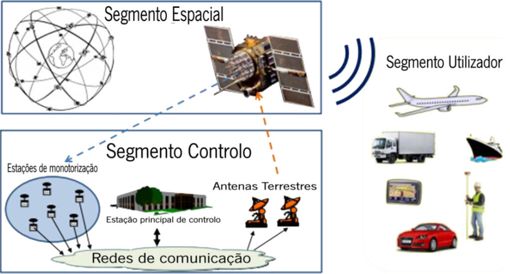
2.1.1 Spatial segment
The GPS spatial segment is composed of satellites that move in medium orbit MEO (Medium Earth Orbits). These satellites are distributed in six orbital planes, located at an altitude of approximately 20,200 km, with four satellite units per orbital plane (Monico, 2008).
Its signals are characterized by the emission of three carrier waves: L1 (1,575 MHz), L2 (1,227.60 MHz) and L5 (1,176.45 MHz). Ionospheric effects are corrected from the simultaneous reception of these carrier waves in the receiver (Monico, 2008).
There are currently three types of signals involved in GPS: the carrier waves specified in the previous paragraph (L1, L2 and L5), the codes (C/A, L2 and P) and data like navigation, clock, among others (Polezel, 2010).
2.1.2 Control segment
The control segment of a GNSS is responsible for continuous monitoring and maintenance, as well as determining their timing system. From this segment on, the satellite clocks are corrected, navigation messages are updated and their ephemeris are predicted, such as orbit inclination and eccentricity of the orbital ellipse, among others (Monico, 2008).
2.1.3 User segment
User segment is the utility component of the systems, and is associated with the receivers of the satellite signals. These receivers are differentiated by usage modes, such as navigation and geodesy, for example. In general, this section is subdivided into two parts: military and civilian. Among the different systems, the user segment is closely related to the different types of existing receivers. Generally speaking, receivers are composed of an antenna with pre-amplifier, radio frequency (RF) section for signal identification and processing, microprocessor for receiver control, oscillator, user interface, power, and data memory (Monico, 2008).
2.2 Ionospheric correction
Measurements, such as topographical ones, or simply as those made with tape measurer or ruler, might carry errors, whether systematic, random, or coarse. Regarding a GNSS there is no difference, but such errors may be corrected. The systematic ones may be reduced or parameterized through observation techniques, as well as the coarse ones. The random ones, on the other hand, are considered inherent properties of the observation, and may remain even after the correction of any other errors (Monico, 2008).
Regarding GNSS systematic errors, four sources of discrepancies may be highlighted. The satellite is one of them, which may cause orbit and clock inaccuracies. The satellite signal propagation is exposed to effects caused by tropospheric and ionospheric refraction, in addition to those generated by multipath or reflected signals, among others. The receiver is subject to interchannel error and delay between two carriers. Finally, satellite signal receiving stations are exposed to the effects caused by atmospheric pressure (Monico, 2008).
In this study, the error caused by ionospheric refraction for single and dual frequency receivers was addressed more specifically, and then a comparison between the two types of equipment was made.
The GPS signals, on their way between the satellite and the receiving antenna, propagate through several layers with different characteristics. The presence of ionised particles (ions and electrons) in the ionosphere makes it a dispersive layer, which affects the modulation and phase of the carrier wave and causes deviation of the signal propagation time from the speed of light. This deviation is also directly related to the frequency of the signal passing through the ionospheric layer and the Total Electron Content. (de Aguiar & Camargo, 2006).
The concentrations of ions and electrons in the ionosphere is a function of space, representing their density, are subject to temporal variations. Such changes are diurnal and seasonal variations. The diurnal changes occur more significantly at low latitudes. In the case of Brazil, its maximum value occurs between 15:00 and 19:00 UTC (Monico, 2008).
After sunset and during the night period until midnight, a phenomenon known as plasma bubble or ionospheric bubbles occurs (Monico, 2008). This phenomenon is directly related to the increase in the occurrence of ionospheric scintillations, which are responsible for the degradation of navigation signals such as GPS (Matsuoka, 2007), consequently causing a delay of the satellite carrier waves when they propagate through the ionosphere. This phenomenon occurs more frequently at high latitudes and in equatorial regions, and can extend throughout the night in some phases of the year (Monico, 2008).
Regarding the medium of signal propagation, the focus of this study remains to that in the ionospheric layer. This variation depends on the atmospheric refractive index, which is proportional to the TEC and inversely proportional to the carrier wave frequency (Monico, 2008).
To better illustrate the relationship of the TEC with the first, second and third order effects in the ionospheric layer on the GNSS observables, the equations for the phase observables follow (ΦLi) and pseudodistance (PDLi) in the band Li (i = 1, 2) incorporated with the effects of the ionosphere in its three orders and can be described as follows:
|
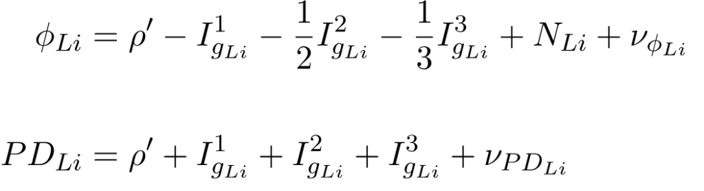
Where ρ‘ represents the satellite-receiver geometric distance plus troposphere effects, clocks, among others. The terms I1gLi, I2gLi and I3gLi and represent the 1st, 2nd and 3rd order group ionospheric effects, respectively. The phase ambiguity is represented by N and the terms 𝝊ϕLi and 𝝊PDLi represent random and unmodeled effects in the phase and pseudodistance equations, respectively. The effects of the three orders can be described in mathematical expressions as follows:
|
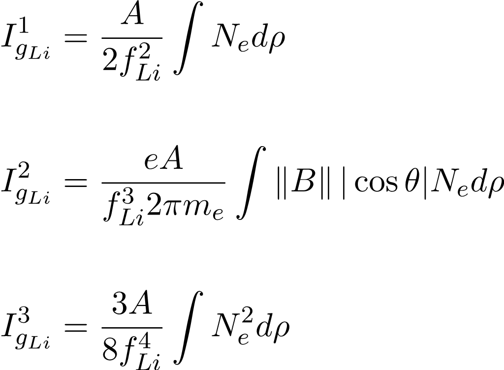
From the equations, it is observed that A = e2 /4πmeɛ0, Ne is the density of free electrons in m-3, e = 1.6021810-19 Coulomb for the charge of the electron, m = 9.1093910-31 kg for the mass of the electron and ε0 = 8.8541910-12 Farad/meter for the permittivity of free space. The B term represents the geomagnetic induction vector (Marques et al., 2009).
Thus, the deviation caused in the ionosphere is linked to the amount of electrons present in the signal path between satellite and receiver, while the TEC varies according to the variation of incident solar radiation (Monico, 2008).
The electron density also changes based on the seasons of the year. At equinoxes, the ionospheric effects are more significant, while at solstices, they reach their lowest levels. As for the geographical factor, the electron concentration varies latitudinally (Monico, 2008). The equatorial regions have high levels of ionospheric density, while in the mid-latitudes, low levels are observed. In turn, the poles are regions of greater difficulty in prediction (Webster, 1993). Such variation with latitude is linked to the zenith angle of the sun, which influences the level of radiation and directly affects the electron density in the atmosphere (Monico, 2008). Based on this quantification, the level of ionospheric anomalies may be determined.
As a last influence on the signal propagation through the ionosphere, remains the effect generated by ionospheric scintillation. Scintillation is noted during the propagation of radio waves in a region with irregularities in the electron density. Currently, ionospheric refraction is responsible for the largest source of error in single frequency GNSS receivers (Dallagnol, 2019). As a result of scintillation, the radio signal may reach the GNSS receiver with reduced intensity, and even be lost completely in some cases (Webster, 1993).
The effect of ionospheric refraction (ionospheric error) may be better estimated from dual frequency receivers data (Monico, 2008). The solution of the ionospheric effect is performed from a linear combination between the two observables (pseudodistance and phase of the carrier wave) at different frequencies, in order to obtain the differences in distance and phase of the carrier wave, with the aim of applying later corrections to the positioning data, correcting them (Seeber, 2003).
Given the above, it is observed that most GNSS use two carriers with different frequencies (Monico, 2008), reaching up to three different carriers, such as GPS, with the implementation of the L5 band.
It is worth highlighting the models used for correction of the ionospheric effect that are generally categorized as an empirical model or a model of mathematical functions. The first is based on data observed in long-term records and represents the characteristic variation patterns, while the second is adjusted by mathematical functions and uses the actual measured ionospheric delay of a given area over a period of time. The Klobuchar model corrects for ionospheric delay by transmission ephemeris, it is only suitable for the mid-latitude area. The NeQuick model is a time-dependent ionospheric electron density and three-dimensional model and is applicable for real-time single-frequency correction. NTCM is a user-friendly TEC model that covers all levels and a global scale of solar activity. This empirical approach describes the dependencies of TEC/ionospheric delay on geographic location, local time and solar irradiation and activity. The GIM (Global Ionosphere Map) assumes that the ionosphere is composed of a thin spherical layer at a height of 450 km above the Earth’s surface. The GIM reconstructed from the predicted and actual measured datasets can be used for real-time and post-processed applications respectively (Hoque et al., 2019).
2.3 Single, dual and triple frequency receivers
Due to its occurrence in a dispersive way, the signal propagation in the ionosphere is directly linked to its frequency, also regarding the velocity reduction this wave propagation through the ionosphere (Monico, 2008).
The ionospheric error may be estimated from phase measurements collected by dual frequency receivers, with the corrections then applied to the single frequency receiver used in the area. This error may also be estimated by the NeQuick and Klobuchar mathematical models. The latter being the best known, applying a correction of up to 60 % in the ionospheric error. This model delivers the values corrected for the delay time due to the ionospheric layer present (Silva, 2020).
The application of triple frequency receivers became notorious with the modernization of GPS. Among its applications is the correction of cycle loss, which is characterized by being a discontinuity in the integer number of cycles in the carrier wave phase (Mendonça, 2019). This interruption is caused by a momentary loss of signal during tracking and stems from factors such as physical obstructions, low satellite elevation angle, and ionospheric scintillation (Seeber, 2003).
In order to achieve higher positioning accuracy in triple frequency receivers, cycle losses must be detected and subsequently corrected. Detection and correction are possible by techniques such as triple phase difference (Mendonça, 2019), discussed later on this text. Detection aims to identify the occurrence of cycle loss, while correction determines the error value. Based on algorithms, it is possible to perform the correction of positioning errors, highlighting the dual and triple frequency sensors, more effective in cycle losses corrections that may be caused by ionospheric effects.
The observations errors may be reduced by the difference between the observables of the tracking stations; these differences give rise to the so-called simple, double and triple differences (Penha & Orihan, 2013).
3 Data and methodology
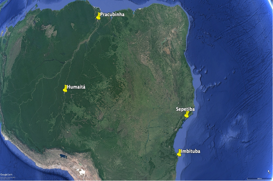
The data analyzed in this paper was extracted from the CHM (Navy Hydrographic Center) database, obtained from static relative surveys performed in Pracubinhas (State of Pará), Humaitá (State of Amazonas), Sepetiba (State of Rio de Janeiro) and Imbituba (State of Santa Catarina), with the objective of evaluate the ionospheric refraction influence over different regions of Brazil. The locations are distributed amongst different latitudes, providing more diversity to the analysis according Fig. 2. Two of the four points are located in the Amazon region due to the higher probability of ionospheric effects in this region, by its location at low latitude. The observables were acquired at frequencies L1 and L2 of the GPS carriers. The Brazilian Continuous Monitoring Network (RBMC) endowed of geodetic stations, was adopted as base stations. The sites used were “AMPA”, located in Macapá, “AMHA” located in Humaitá, “CHPI” located in Cachoeira Paulista, and “IMBT” in Imbituba. The established data recording period was 15 seconds with an elevation mask of 15°, standards suggested in the DHN Technical Instructions.
The data were collected as DL-V3 receiver’s own format, generating data with “.pdc” file extension. For the data to be in the appropriate format for processing, they were converted to the RINEX format (https://www.igs.org/wg/rinex/#documents-formats). The conversion may be carried by the “NovAtel convert” software or the application “RTKconv”, the latter being one of the components of the software RTKLib (Real Time Kinematic Library), version 2.4.2.
The data processing in RINEX format was performed by means of the application “RTKpost”, which is part of the software RTKLib version 2.4.2. At the end, a file in “.txt” extension is generated, with relevant information such as the standard deviations of the positioning data obtained by tracking.
The RTKLib software uses the Klobuchar model for ionospheric refraction correction. This model is applied to the correction of ionospheric refraction in single frequency receivers (Dallagnol, 2019). Klobuchar model was developed for mid-latitudes and therefore produces the best correction of the ionospheric error for single frequency data. The information from the navigation message is applied to a polynomial estimated from a network of global GPS stations (Dallagnol, 2019). The model considers the total electron content (TEC) as a thin layer of the atmosphere (Dallagnol, 2019). Thus, it considers the multiplication by an obliquity factor for the signal delay suffered in the ionosphere, which reduces the ionospheric error by about 60 % (Dallagnol, 2019).
For data analysis in the present paper, the ionospheric correction mode was deactivated, aiming a better comparative analysis of the ionospheric effect correction in dual frequency receivers, compared to single frequency ones.
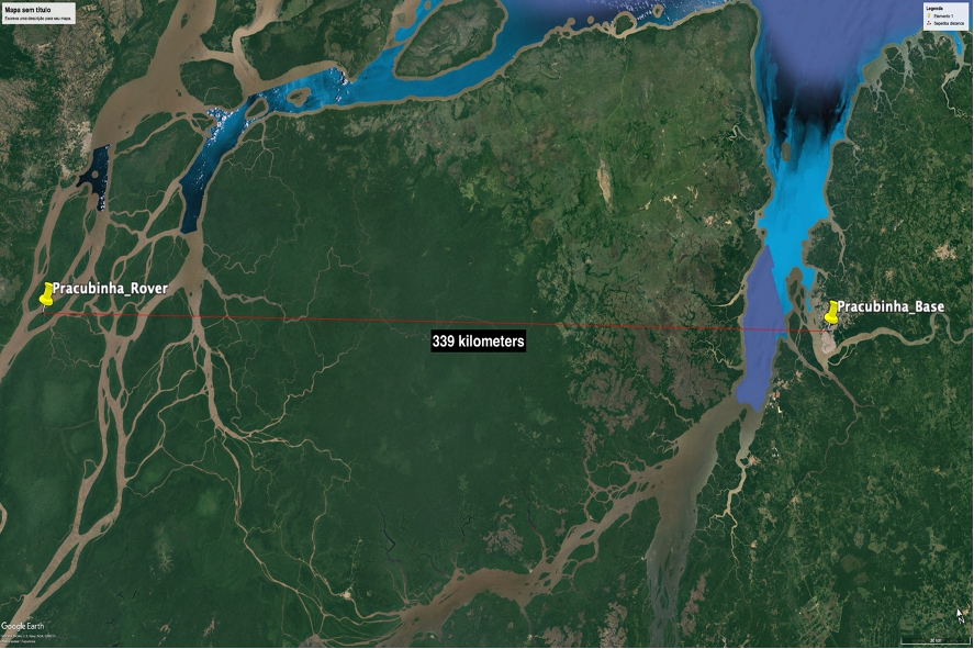
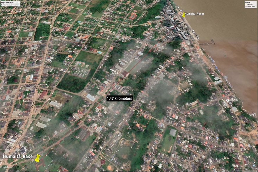
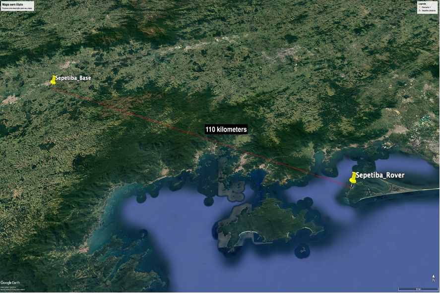
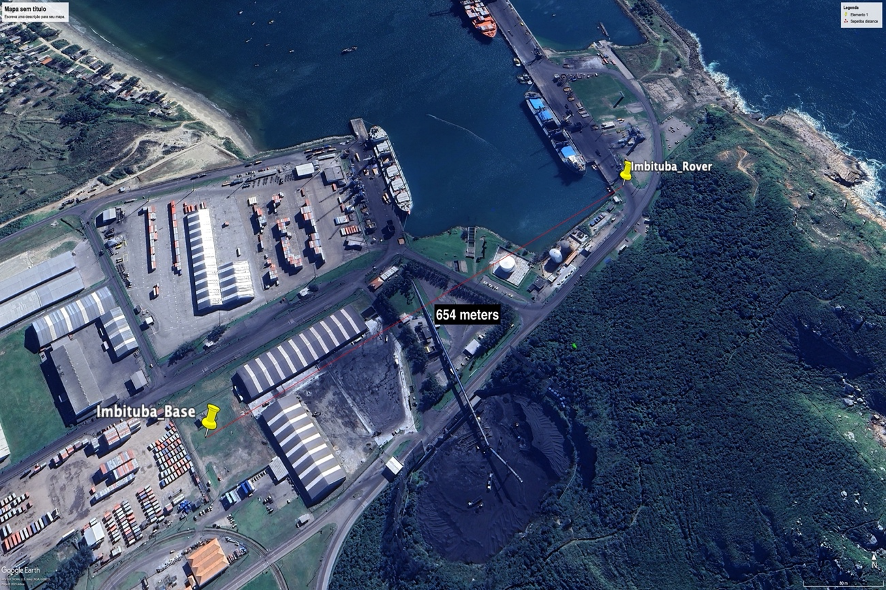
The files processed were collected at double frequency, using the static relative positioning method. After the conversion to RINEX format, only the data referred to the observations were used, without the application of satellite navigation data. As reference information, the positioning data (in RINEX format) from the RBMC stations were employed. These base station data are available on the Brazilian Institute of Geography and Statistics (IBGE) internet site. Illustrations with the lengths of the baselines that connect the base station to the rover station of the tracking points in pracubinhas, humaitá, sepetiba and imbituba, can be found in Fig. 3, 4, 5 and 6 respectively. Finally, precise ephemeris and clock corrections, provided by the international GNSS service of NASA (National Aeronautics and Space Administration), were added to the processing.
All the data described above were also processed in the RTKpost application. The processing was done first in single frequency and then in dual frequency mode. The evaluation was based on the analysis of the standard deviation of the positioning over time, in the X-, Yand Z-axes for a geocentric coordinate system.
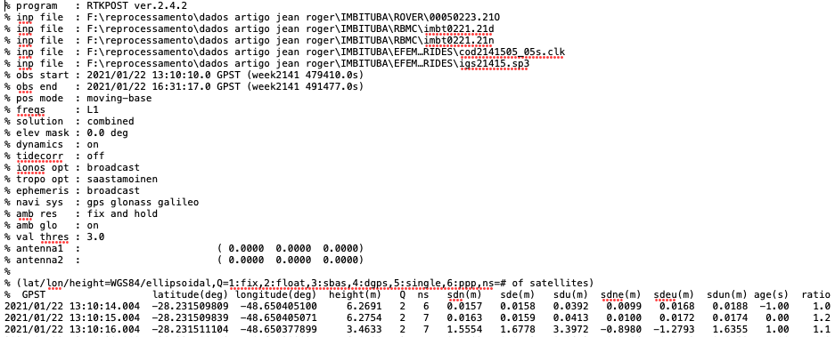
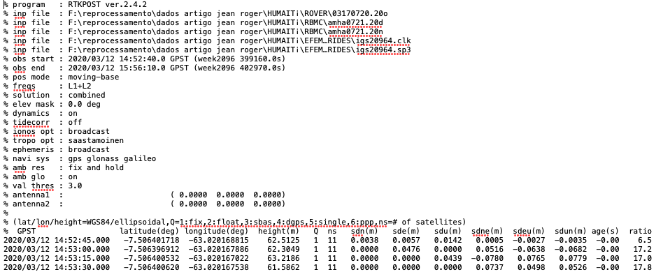
Annexes A and B, display parts of the positioning solution files obtained with the software RTKLib in frequency L1 (single frequency) and in frequencies L1 and L2 (dual frequency). These files come from the same tracking, processed separately by frequency (single and dual).
The data were collected with a 15 second interval for approximately four hours. With the application of the tools available in the RTKlib software, it is possible to obtain graphs of the standard deviation of position as a function of time, displayed in a scatter plot, as well as discriminate when the receiver obtained solutions was on “float” or “fix” mode. The confrontation of the quality of such solutions in each of the processing procedures, contributed to the evaluation between the generated products.
4 Results and discussion
As an outcome of each data processing by the RTKpost application, a report is generated with the calculated positioning solutions. This report is in “.txt” format according to annexes A and B, and may be described as follows: lines beginning with the character “%” describe the header of the file. The penultimate line beginning with “%” shows that the latitude, longitude and altitude were based on the WGS-84 reference system. The variable “Q” stands for Quality Flag, as stated in the RTKLib 2.4.2 manual, and may have one of the following values:
- Fixed point – Ambiguity and positioning of the point of interest is solved.
- Float – Position solution provided by the base, but the ambiguity is not entirely solved.
- SBAS (Satellite-Based Augmentation System) – Positioning with differential correction provided by geostationary satellites (Albarici, 2011).
- DGPS – Position with differential GPS corrections or SBAS corrections.
- Single – Absolute positioning.
- PPP – Precise Point Positioning.
In sequence, “ns” corresponds to the number of satellites used to estimate the positioning solution. The RTKplot application provides as outputs, the graphs of the positioning standard deviation as a function of time. It should be noted that these graphs are arranged in three parts, from top to bottom, with illustrations of the standard deviations in x, y and z respectively, as a function of time.
The results obtained were also illustrated in scatter plots. This aimed to illustrate the difference between outputs generated for single and dual frequency processing.
In order to exclude the possibility of satellite geometry affecting the results, the same satellites (number and PRNs) are used for the single frequency and dual frequency solutions, at each tracking location, changing only the processing mode (single frequency and dual frequency) aiming to compare both methods.
4.1 Static positioning at Imbituba-SC
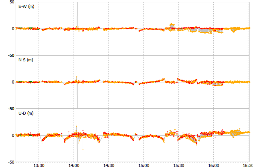
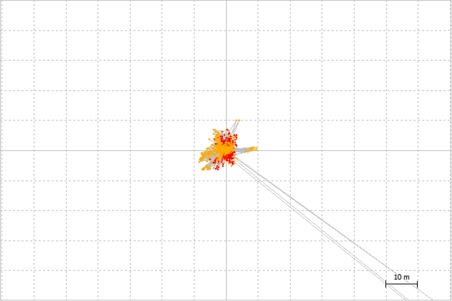
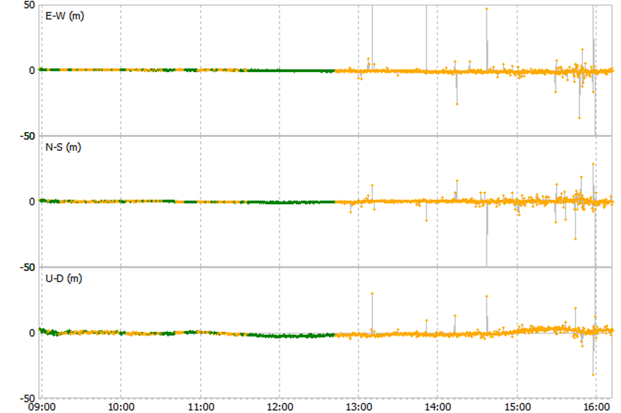
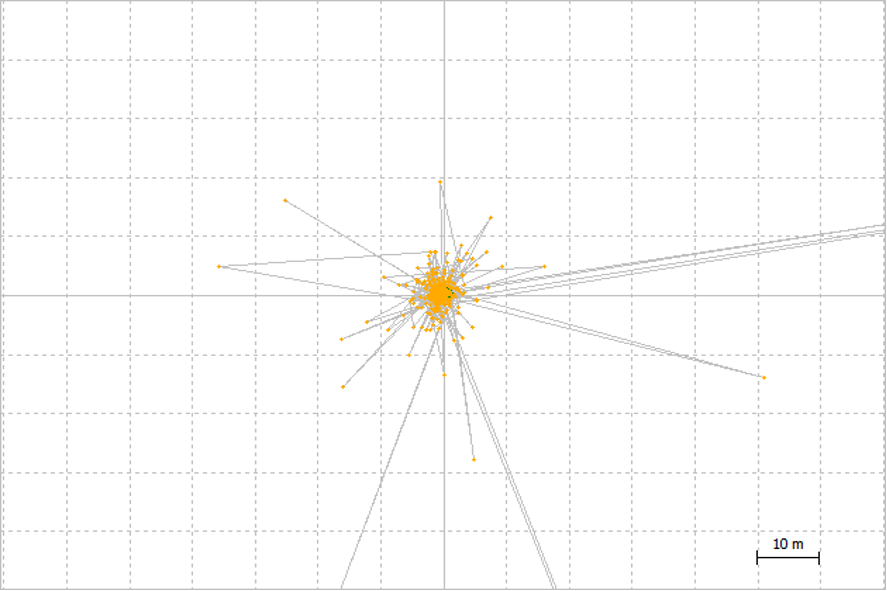
The data at Imbituba was collected on 01/22/2021, between 13:10:10 hour and 14:31:17 hour UTC. The single frequency data processing results for the standard deviation as a function of time, are shown in Fig. 7 as a two colors graph. The orange line, corresponds to the float solution, and the red one, from single solution. There were no positions evaluated as fix over time, which indicated the absence of good position solutions in the survey and, consequently, the absence of adequate positioning accuracy. Spurious data peaks were observed between 14:00 hour and 14:15 hour, as well as between 15:15 hour and 16:00 hour. These occurrences are displayed in Fig.8, which shows the scatter plot of the data collection, with points that are out of sync with the receiver location.
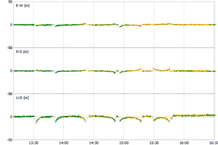
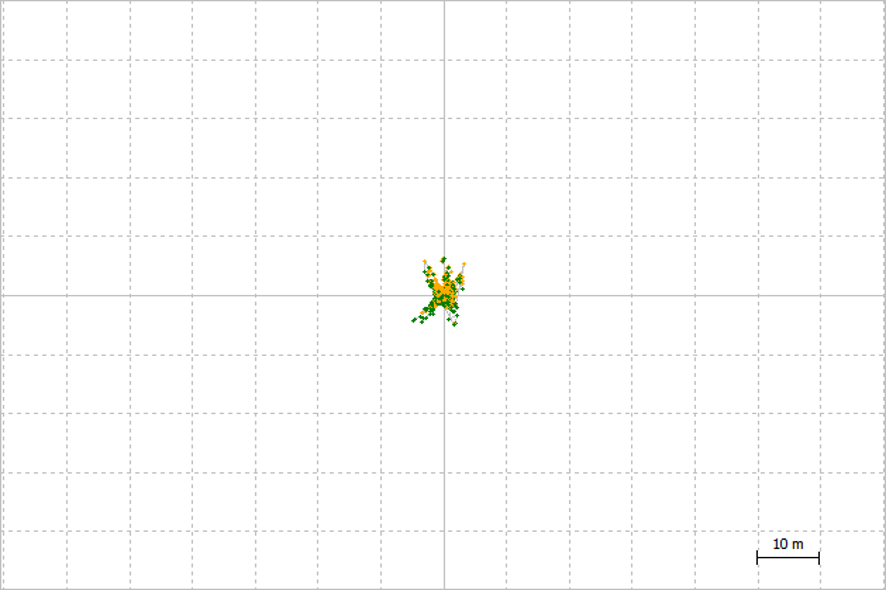
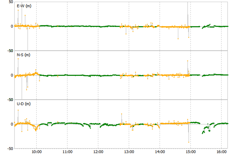
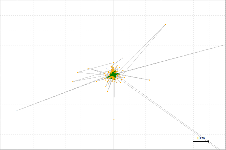
In Fig. 9 and 10, there is evidence of a marked improvement in the positioning solution with dual frequency data processing. In Fig. 9, the graph of the standard deviation as a function of time provides a large amount of green data, corresponding to the “fix” solution. On the other hand, an increase in the occurrences of “float” results is observed after 15:15 hour, but still with the presence of “fix” solutions. These results corroborate the expected effects in surveys carried close to sunset, when the ionospheric refraction has a greater effect on positioning (Caldeira, 2016). The comparison of the two processing methodologies also shows a smaller variation of the positioning standard deviation, for a dual frequency processing. This dispersion, less expressive, is presented as a cloud of points more concentrated around the point actually occupied (Fig. 10), which denotes greater accuracy of the results.
4.2 Static positioning in Sepetiba-RJ
The field data in Sepetiba-RJ were acquired on 11/13/2018, between 20:57:45 hour and 16:12:45 hour UTC.
The results observed in Imbituba show a larger amount of “fix” solutions for dual frequency processing. Again, particularly for the afternoon period, when the difference regarding the single frequency processing is notorious (Fig. 11 and 13). The variation in the standard deviation, less expressive, points to greater accuracy in positioning, in accord with the greater number of “fix” solutions in the collection. It is also possible to note this evidence in the scatter plots (Fig. 12 and 14).
4.3 Static positioning in Pracubinhas-PA
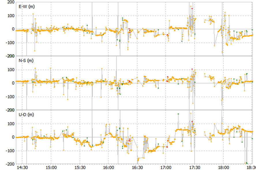
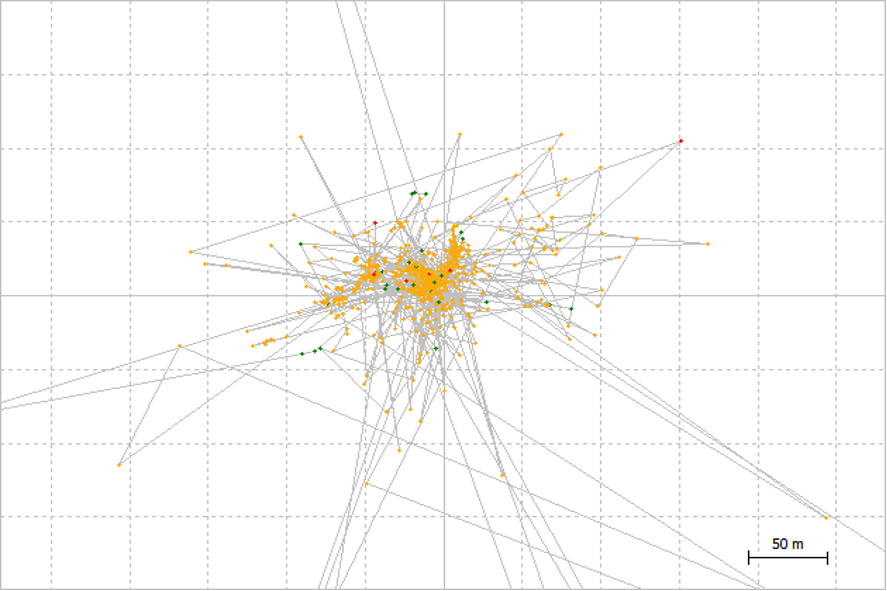
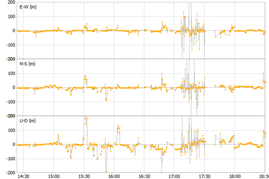
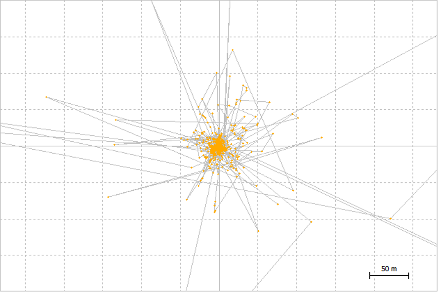
In Pracubinhas-PA, the static survey was performed between 14:23:25 hour and 18:33:10 hour UTC, on 02/26/2019.
Once again, it is observed, with more prominence between 15:15 hour and 16:45 hour, the position solution for mono frequency with more expressive variation of its standard deviation, when compared to the dual frequency data, as indicated in Fig. 15 and 17 The different dispersions of the scatter plots, referring to the two processing methods, demonstrate the positioning accuracies obtained, as may be seen in Fig. 16 and 18.
4.4 Static screening in Humaitá-AM
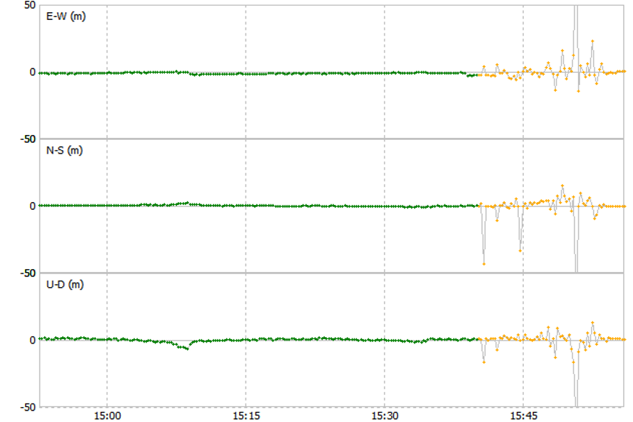
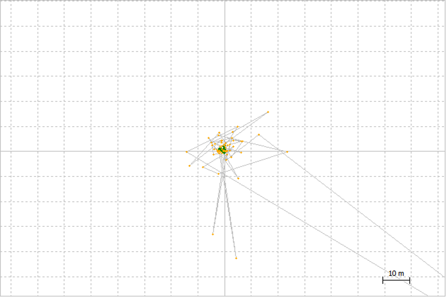
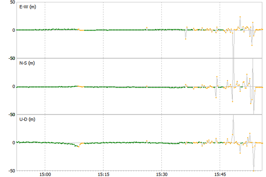
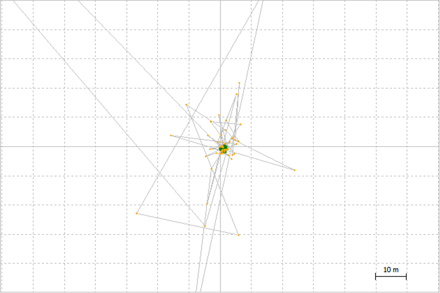
The analysis of the positioning solution for Humaitá-AM data obtained on 12/03/2020, between 14:52:40 hour and 15:56:10 hour, UTC. When considering the uncertainty measures illustrated in Fig. 19 and 20, it is observed that the positioning quality degradation occurs faster in single frequency positioning. Even if it was caused by some local factor, such as physical obstruction and consequent multipath, it was possible to notice that when using the dual frequency, the information quality was maintained for a longer period. The “fix” outcomes were more often for dual frequency data, which denotes greater accuracy in the positioning solution, compared to the single frequency solution. Thus, it is observed a higher scatter points concentration in Fig. 22, which illustrates positions by dual frequency, when compared to the Fig. 20, stating the higher positioning quality of dual frequency data.
5 Conclusion
Researches focused on the study of ionospheric effects on satellite positioning data are extremely important in the case of Brazil, which is located in an equatorial/tropical region, where the ionospheric effects are stronger.
It has been shown in this paper that the ionospheric error presents a reduction in its effects when satellite data is collected with dual frequency receivers. Currently, the determination of ionospheric refraction has been done from models that use observations received by dual frequency GNSS receivers. In them, the systematic error caused by the ionosphere is estimated, and then its correction is applied in single frequency receivers (de Aguiar & Camargo, 2006).
Aiming a larger diversification in data analysis, the selected survey spots were located in different latitudes. In all, four stations evaluated, two of them are at low latitude (Amazon region) due to the higher probability of the ionospheric error occurring. No major distinctions were observed in outcomes from the processed data from southern and southeastern regions when compared to the northern region results.
It was observed in the interval between 15:00:00 hour and 16:00:00 hour UTC, the recurrence of spurious data in standard deviation graphs as a function of time, being an indication of the occurrence of ionospheric error, on account of sunset proximity which favors the ionospheric refraction increasing. The sunset at each tracked point is: Imbituba: 20:13 hour, Sepetiba: 18:06 hour, Pracubinhas: 18:28 hour and Humaitá: 17:58 hour. The occurrence of other types of interference on the satellite signal carrier, such as multipath or cycle slips is not ignored, but assigned to the recurrence of signal degradation for the same time interval for stations at different latitudes, there is a strong indication that this degradation has been influenced by the ionospheric effect. Similarly, an improvement in the positioning data accuracy for this specific day period was observed when the processing was carried out with double frequency. Particularly for Humaitá-AM station, where the application of dual-frequency processing indicates a longer period of “fix” solution classification, compared to single frequency positioning. This aspect indicated not only an improvement of positioning accuracy, but also a shorter time to achieve it when performing dual frequency positioning.
References
Albarici, F. L. (2011). Posicionamento relativo: Análise de resultados combinando observáveis L1 de satélites GPS e SBAS. Dissertação apresentada à Escola
Caldeira, Mayara Cobacho Ortega (2016). Análise do Impacto do Efeito Ionosférico e Cintilação Ionosférica no Posicionamento Baseado em Redes e Por Ponto. Dissertação apresentada ao Programa de Pós-Graduação em Ciências Cartográficas da Faculdade de Ciências e Tecnologia da Universidade Estadual Paulista “Júlio de Mesquita Filho”. https://repositorio.unesp.br/ bitstream/handle/11449/144291/caldeira_mco_me_prud.pdf?sequence=3&isAllowed=y (accessed 14 March 2023)
de Aguiar, C., and Camargo, P. (2006). Real Time Modeling of the Systematic Error in GPS Observables Due to Ionosphere. Bulletin of Geodetic Sciences, 12(1). https://revistas.ufpr.br/bcg/ article/view/5307
Mainul, M. and Jakowski, N. (2012). Ionospheric Propagation Effects on GNSS Signals and New Correction Approaches. InTech. doi: 10.5772/30090
Martins, F. V. I. (2016). Sistema de Aquisição e Teste de Sinais GNSS para Condução Autónoma. Dissertação de mestrado em Engenharia Eletrónica Industrial e Computadores. Braga, Portugal. https://hdl.handle.net/1822/46633
Mendonça, C. H. C. (2019). Detecção e Correção de Perdas de Ciclos Para Dados GPS de Tripla Frequência. Dissertações Ciências Cartográficas – FCT. http://hdl.handle. net/11449/183236
Monico, J. F. G. (2008). Posicionamento pelo GNSS: descrição, fundamentos e aplicações. UNESP.
Penha, J. W., and Orihan, M. (2013). Mapas do efeito ionosférico nas observáveis GPS pelo parâmetro VTEC no declínio do ciclo de manchas solares no Brasil. In: XVI SBSR -Simpósio Brasileiro de Sensoriamento Remoto, Foz do Iguaçu -PR. Anais do 16º Simpósio Brasileiro de Sensoriamento Remoto. São José dos Campos -SP: MCT/INPE, p. 1899–1907.
Polezel, W. G. C. (2010). Investigações sobre o impacto da modernização do GNSS no Posicionamento. 106 f. Dissertação (mestrado) Universidade Estadual Paulista, Faculdade de Ciências e Tecnologia. http://hdl.handle.net/11449/86810
Seeber, G. (2003). Satellite Geodesy: Foundations, Methods, and Applications (2nd ed.). Walter de Gruyter. https://doi. org/10.1515/9783110200089
Silva, J. R. (2020). Uma Análise Do Modelo De Klobuchar Para Avaliação De Erros Ionosféricos. São José dos Campos: INPE, 20 p. Bolsa PIBIC/INPE/CNPq. IBI: 8JMKD3MGP3W34R/442HJ3E. http://urlib.net/ibi/8JMKD3MGP3W34R/442HJ3E
Annexes
Authors’ Biographies

Lieutenant J. Roger da Silva, Navigator of Hydroceanographic lighthouse keeper Vessel “Almirante Graça Aranha” (Brazilian Navy). B.Sc. in Naval Science (Naval College, 2017). He completed the Hydrographic Course IHO/FIG/ICA Category A in 2021 (Directorated of Hydrography and Navigation – DHN).

Guilherme A. G. do Nascimento was born in Niterói-RJ. Lieutenant Commander of the Brazilian Navy, earned a bachelor’s degree in Naval Sciences from the Navy Academy (Escola Naval), a Specialization in Hydrography from the Directorate of Hydrography and Navigation (DNH -Diretoria de Hidrografia e Navegação) and holds a master’s degree in Cartographic Sciences from the Paulista State University (Universidade Estadual Paulista). He has worked on hydrographic surveys through the Brazilian coast and in the Amazon region and is currently head of the Topogeodetic Information Section (Seção de Informações Topogeodésicas) of the Navy Hydrography Center, (Centro de Hidrografia da Marinha), in Niterói-RJ.