


Abstract
1 Introduction
Sea Surface Salinity (SSS) provides information on the concentration of dissolved salts in the upper centimeter of the ocean surface. It is a key parameter that contributes to global ocean circulation and the earth’s climate, as well as providing fundamental information for ocean biogeochemistry (Fine et al., 2017; Land et al., 2015, 2019; Siedler et al., 2001; Wang et al., 2022). Hence, it can affect marine ecosystems (organisms and plant community), the physical properties of the oceans (temperature, density, pressure, waves, and currents), as well as the water cycle and ocean circulation (Jang et al., 2022; Pradesh, 2019). Importantly, salinity in conjunction with temperature determines seawater density, which in turn drives many ocean processes such as vertical mixing, double diffusion, horizontal circulation, and near-surface stability. Salinity also plays a crucial role in modulating the air-sea interaction (surface fluxes of heat and CO2) due to its impact on boundary layer processes. Hence, even small variations in SSS can have dramatic effects on the ocean system. Furthermore, the ocean water freezing point also depends on salinity (it takes longer for more saline water to freeze than less saline water). Thus, making the investigation of salinity variation imperative.
There is a wide range of spatiotemporal variations in the distribution of salinity within the oceans, seas, and lakes, even though the relative abundance of the major salts in seawater is largely constant. This variation is both horizontal and vertical. Sea surface salinity is mainly controlled by the balance between evaporation and precipitation. Hence, high salinity concentrations are recorded in the regions around 20° to 40° North and South (sub-tropical central gyre regions), where evaporation is extensive, but rainfall is minimal. Globally, the average salinity in the oceans and the seas is 35‰ (Droppleman et al., 1970; NASA, 2022).
Due to the importance of sea salinity in global water balance estimation, evaporation rates, and ocean currents, it is crucial that salinity is continuously monitored to have a good understanding of its variability and potential impacts on ocean process and water balance. While some parts of the world are currently experiencing increasing salinity levels, others are experiencing decreasing salinity. For instance, the Arctic is experiencing an increase in temperature (IPCC, 2018), which is modifying the freshwater cycle in the region and leading to decreasing salinity (Carmack et al., 2016). However, in the Barents Sea, which is also within the same Artic region, both temperature and salinity are increasing due to the increase of salty water supply from the North Atlantic waters, that is the so-called ‘Atlantification’ (Lind et al., 2018). Such changing dynamics in salinity variation demonstrate the need for continuous monitoring of SSS variation, to facilitate understanding of the underlying factors triggering this and their potential impact. This is especially important with increasing climatic changes that may further alter salinity concentrations across the oceans (Bindoff et al., 2019). Changes in ocean salinity concentrations could significantly alter local salinity regimes, which in turn could affect ecosystem composition in nearby communities, as well as altering interactions between organisms. This would have profound effects on communities in developing countries, especially those in West and Central Africa with much reliance on ecosystem services from the marine environment (ocean, estuaries, and fresh waters). This could have significant effects on the local economy by affecting fishing industry, reducing freshwater availability (water quality), as well as soil salinity imbalances that could affect food security. In addition, varying salinity concentrations could alter species distribution marine, estuarine, and freshwater species, although the magnitude of the impacts depends on the underlying physiology and tolerances of organisms and their ability to cope with salinity fluctuations on both long-and short-time scales (Smyth and Elliott, 2016).
Hence, within the past two decades, salinity variations across the global seas and oceans have regularly been observed by satellites (Boutin et al., 2021; D’Addezio et al., 2019; Fournier et al., 2015; Gierach et al., 2013; Grodsky et al., 2012; Jang et al., 2022; Korosov et al., 2015b; Lagerloef, 2012; Lee et al., 2012; Melzer & Subrahmanyam, 2015; Rani et al., 2021; Reul et al., 2020; Reul et al., 2014; Supply et al., 2020). Deployment of satellite methods enabled consistent measurement of weekly, monthly, interannual, and decadal variations in salinity. Currently, sea surface salinity values derived from various satellite sensor data are enabling widescale routine monitoring of salinity variability, seawater plumes, and climate change on global, and regional scales.
Despite having been collected by various satellite sensors for over a decade, sea surface salinity measurement is not regularly available to many users, especially researchers in developing countries, or to non-remote sensing specialists who lack the necessary skills and tools to extract these data from satellite data. This limits the extensive study and wider understanding of the spatiotemporal variations of ocean salinity in many areas and their attendant impact on the marine environment and climate change. Due to the importance of the oceanic environment, some projects have been dedicated to alleviating access to key oceanic variables to interested parties. The Copernicus Marine Service is a key program of the European Union, is one of such projects that is used to provide free, regular and systematic information on the state of the ocean (including salinity), on a global and regional scale. However, users are constrained to only data available on the visualization platform, some of which are presented at a relatively coarse spatial resolution (e.g. Global Ocean- Real time in-situ observations objective analysis product presented at a 0.5 degree spatial resolution) (Szekely, 2022). Hence, in this study, we aimed to develop an automated approach (End-to-End Extract, Transform, Load, and Report (ETLAR) data pipeline) to extract sea surface salinity from satellite data. Using the developed method, we investigated the spatiotemporal variation of ocean salinity across the western coast of Africa. We set out to achieve the following key objectives: develop an automated technique for easy and quick retrieval of salinity data from satellite data into commonly used data format, investigate and map spatiotemporal variations of sea surface salinity across the western coast of Africa, identify spatial and longitudinal trends and pattern in SSS in the region, and create sea surface salinity data store and visualization service to facilitate easier access to data, interrogation of SSS data, and routine reporting of salinity variations in the study area.
2 Variation of sea surface salinity
The horizontal distribution of ocean salinity is conventionally studied in relation to latitudes. Generally, salinity decreases from the equator towards the poles. However, the highest salinity concentration is hardly recorded near the equator despite the fact that this zone records high temperature and evaporation. This is due to high rainfall activity in this zone that reduces the relative proportion of salt in the waters. Thus, salinity around the equator is roughly around 35 ‰. The highest salinity concentrations are generally observed between latitudes 20°–40° N (36 ‰) because this zone is characterized by high temperature and evaporation rates, with relatively low rainfall. The average salinity of 35 ‰ is recorded between latitudes 10°–30° S in the southern hemisphere. The zone between 40°–60° latitudes in both hemispheres records low salinity (31 ‰ in the northern hemisphere) and (33 ‰) in the southern hemispheres. Salinity further decreases in the polar zones because of the influx of meltwater (Antonov & Levitus, 2006).
2.1 Key factors controlling SSS
The key factors controlling sea surface salinity include evaporation, precipitation, the influx of freshwater (from rivers), ice melts, atmospheric pressure, wind direction, and circulation of oceanic water (Durack et al., 2012; Qu et al., 2014; Skliris et al., 2014). Salinity positively correlates with the rate of evaporation (the greater the evaporation, the higher the salinity concentration and vice versa). Evaporation due to high temperature with low humidity (dry condition) causes higher salinity levels. Hence, salinity is higher near the tropics than at the equator because although both the areas record a high rate of evaporation it is less humid (dry air) over the tropics of Cancer and Capricorn.
Precipitation is inversely related to salinity (higher volumes of precipitation result in lower salinity and vice versa). High-frequency rainfall events can substantially affect salinity concentration on varying spatial scales (Akhil et al., 2016; Boutin et al., 2016). Therefore, the regions of high rainfall (equatorial zone) generally, record comparatively lower salinity than the regions of low rainfall (sub-tropical high-pressure belts). It may be simply stated that the volume of water in the oceans is increased due to heavy rainfall and thus the ratio of salt to the total volume of water is reduced.
Furthermore, meltwater from the polar areas supplies extra water in the temperate regions that increase the volume of water and therefore reduce salinity. Hence, the impact of ice melt on salinity is noticeable in polar regions, where such processes produce substantial sea surface salinity gradients (Brucker et al., 2014). In addition, the influx of water from rivers also affects the salinity of oceans. Strong river outflow normally causes strong gradients in sea surface salinity (Fournier et al., 2015; Gierach et al., 2013; Grodsky et al., 2012; Korosov et al., 2015a; Reul et al., 2014). Thus, low-salinity concentration usually indicates sources of fresh water, such as rivers and streams that are feeding the ocean (Burrage et al., 2008; Schroeder et al., 2012). Even though such rivers often carry natural and anthropogenic contamination from the land to the sea and can directly impact marine ecosystems with a higher level of salinity, the quantity of water in the inflow normally neutralizes the concentration of salt, thus, leading to an overall reduction of salinity concentration. This is especially noticeable around the mouths of major rivers. For instance, comparatively low salinity is found near the mouths of the River Niger, River Congo, the Amazon River, etc. The effect of the influx of river water is more pronounced in enclosed seas (e.g. the Dniester, the Dneiper, the Danube). This also accounts for the relatively low salinity (17 ‰) in the Black Sea, as it receives an influx from many rivers in Europe. However, in places where evaporation exceeds the influx of fresh river waters, salinity concentration increases (e.g. the Mediterranean Sea records salinity levels of about 40 ‰).
Atmospheric pressure and wind direction are other factors that affect salinity. Anticyclonic conditions with stable air and high-temperature increase the salinity of the surface water of the oceans. Sub-tropical high-pressure belts represent such conditions to cause high salinity. Winds also help in the redistribution of salt in the oceans and the seas as winds drive away saline water to fewer saline areas resulting in a decrease of salinity in the former and an increase in the latter. Ocean currents affect the spatial distribution of salinity by mixing seawaters. Equatorial warm currents drive away salts from the western coastal areas of the continents and accumulate them along the eastern coastal areas. The high salinity of the Mexican Gulf is partly due to this factor. The North Atlantic Drift, the extension of the Gulf Stream increases salinity along the north-western coasts of Europe. Similarly, salinity is reduced along the northeastern coasts of North America due to the cool Labrador Current.
2.2 Historic development in ocean salinity measurement/monitoring
Despite its long-recognized importance, salinity was historically under-sampled across the globe, due to the challenges posed by using traditional methods to measure salinity. Before the deployment of electronic instruments in salinity measurements, accurate salinity measurements relied on complex chemical analysis to precisely determine the salinity content of water samples in laboratories or on research vessels. Hence, salinity observations were very sparse. This was improved through the development of conductivity-temperature-depth (CDT) technology that allowed salinity to be inferred through conductivity measurements. This led to the routine observation of salinity profiles, although observations were still limited in space and time, because of the sparseness of hydrographic sections performed by research vessels. However, the deployment of autonomous Argo profiling float array (Roemmich et al., 1999) improved this situation by enabling routine sampling of high-quality salinity profiles down to 2000m depth on a global scale (Stammer et al., 2021; Stammer et al., 2019; Weller et al., 2019).
Subsequently, various gridded salinity products of the historical data sets (climatologies) such as the World Ocean Atlas (WOA; Antonov & Levitus, 2006; Boyer and Levitus, 2002; Zweng et al., 2018) and EN4 data set (Good et al., 2013) were developed based on historical salinity observations. These are used for salinity and freshwater change studies (Curry et al., 2003; Palmer et al., 2019). Furthermore, numerical ocean models were developed and used in simulating salinity variations and their impacts on ocean processes (e.g., geostrophic flow fields or sea level), using atmospheric forcing fields.
Recent development in satellite remote sensing resulted in the measurement of sea surface salinity from space. This technology is based on inferring surface salinity from satellite sensor measurements of microwave radiance emitted from the top mm of the sea. Detailed technical information on the basic physics of salinity measurement from space, various salinity missions as well as satellite SSS products quality assessment is provided by (Reul et al., 2020). This has led to regular global measurement of sea surface salinity roughly every three days with a relatively high spatial resolution (Vinogradova et al., 2019).
2.3 Satellite monitoring of sea surface salinity
Before the deployment of satellite remote sensing in ocean salinity measurement, SSS was poorly sampled globally. Estimation of sea surface salinity from space began in 2009, following the launch of the Soil Moisture and Ocean Salinity (SMOS) mission. SMOS is one of the European Space Agency’s Earth Explorer missions and provided global observations of variability in two important climate variables: SSS and soil moisture, due to continuous exchange in the earth’s water cycle between the oceans, the atmosphere, and the land. The sensor can detect salinity at 50 km, which is a relatively high spatial resolution (Bell et al., 2004; Glenn et al., 2004; Rani et al., 2021).
Following the success of this mission, NASA, in collaboration with Argentina’s space agency, Comisión Nacional de Actividades Espaciales (CONAE) launched Aquarius in 2011, to study the links between ocean circulation, the global water cycle, and climate. The Aquarius mapped global changes in ocean surface salinity with a resolution of 150 km and 7 days repeat cycle. Hence, provided information on how salinity changes week on week, month on month, season to season, and year to year, until June 2015 when some of the components malfunctioned. The salinity measurement from space was continued with NASA’s Soil Moisture Active Passive (SMAP) satellite. Although SMAP’s mission is primarily focused on the water content of the soil, its highly sensitive radiometer operates on a similar wavelength as Aquarius, and thus, has been used as a replacement for Aquarius, while providing a continuous record of essential information on the ocean, water cycle, and climate. SMAP has a repeat cycle of 8 days with a spatial resolution of 40 km (better than Aquarius). However, SMAP’s 40-km data are noisier than Aquarius data. Thus, some SMAP data products are spatially averaged to larger footprints (60–70 km) to reduce the noise. Due to the success of the missions, various satellite products such as the Optimally Interpolated Sea Surface Salinity (OISSS) products have been developed to combine data from the various missions and process them into a continuous and consistent SSS record.
3 Study area
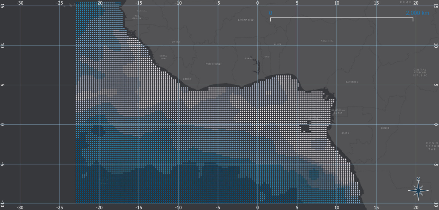
The study area spans the coastal areas of West Africa, between latitudes (15.5° N and 10.0° S) and longitudes (13° E and 23.0° W) as shown in Fig. 1. It cuts across the coast of the following West African countries: Nigeria, Benin Republic, Togo, Ghana, Ivory Coast, Liberia, Sierra Leone, Guinea, Guinea-Bissau, The Gambia, Senegal, and those in Central Africa: Cameroun, Gabon, Equatorial Guinea, Republic of Congo, Democratic Republic of Congo, and Angola. The Equator and Central Meridian pass through the study area, which extended towards the middle of the South Atlantic Ocean. Due to its proximity to the Equator, the bulk of the study area experiences high rainfall and temperature events. However, there are also many rivers such as the Niger, Congo, Sanaga, Rey, Campo, Muni, Volta, Cavalla, Casamance, Gambie, and Geba, flowing into the ocean from most of the countries, which modulate the salinity concentrations in the ocean waters around this area.
4 Methodology
4.1 Data
Data used in this research were sourced from the Multi-Mission Optimally Interpolated Sea Surface Salinity (OISSS) Level 4 dataset, a new global multi-satellite sea surface salinity (SSS) product, made available through the Physical Oceanography Distributed Active Archive Center (PO.DAAC) tool. The product is a combination of data from a suite of satellites (Aquarius/SAC-D, Soil Moisture Active Passive (SMAP) satellite missions, and Soil Moisture and Ocean Salinity (SMOS)), processed into a continuous and consistent 4-day or monthly SSS record. The OISSS product covers the global ocean, including the Arctic and Antarctic areas free of sea ice. However, it does not cover internal seas, such as the Mediterranean and the Baltic Sea.
The dataset used in this research covers SSS acquired from August 2011 to the present. Data from August 2011 to June 2015, were derived from the Aquarius satellite, while the rest are from SMAP satellite-based SSS. The data were processed with Optimum Interpolation analysis on a 0.25-degree grid at a 4-day interval (Melnichenko et al., 2016). A bias correction was applied to the data product to correct the satellite retrievals for large-scale biases concerning in-situ data. Where there is any gap in SMAP data (June–July 2019, when the SMAP satellite was in a safe mode and did not deliver scientific data) SSS data from the ESA’s Soil Moisture and Ocean Salinity (SMOS) satellite were used to fill the gap in SMAP observations. The consistency and accuracy of the new SSS dataset were validated against in situ salinity from Argo floats and moored buoys. The mean root-mean-square difference (RMSD) between the Aquarius/SMAP OISSS dataset and concurrent in-situ data globally is around 0.19 psu and product bias is about zero (Melnichenko et al., 2016). The SSS data in the PO.DAAC tools are provided in network Common Data Form (netCDF-4 format). This is a hierarchical data format, with the metadata included in the data file, thus making it amenable to programming codes.
4.2 Methods
A key aspect of this research is the development of an End-to-End Extract-Load-Transform-and-Report (ETLAR) data pipeline capable of extracting SSS information from the OISSS presented in netCDF-4 data format. To build the ETLAR data pipeline, several automated tools were developed with Python codes for extracting the raw datasets from the PO.DAAC tool, transformation and processing of the extracted data, and analysis, visualizations. Python was chosen because of its simplicity and flexibility in handling different programming tasks. It is a high-level, general-purpose programming language, with dynamic semantics and many built-in libraries, which has made it very attractive for Rapid Application Development (RAD). The interactive reporting dashboard for the presentation of the processed data was built with Power BI. PowerBI is a leading interactive data visualization software product that is freely available. It is a unified and scalable platform for self-service and enterprise business intelligence (BI), its power lies on its ability to integrate and process data from disparate sources and present these with interactives visuals that could draw out underlying trends in the data. It was chosen for this project because it is free, powerful visualization capabilities and ease of deployment of dashboard on the web. The data extraction tool developed with Python was built with the capability to extract the entire global data. However, there was also a provision for it to accept the bounding box coordinates as parameters used in clipping the global data to a specific area. In this research we used the following boundary coordinates to clip the extracted data to the study area (max_lat = 15.5, min_lat = -10.0, max_lon = 13.0, min_lon = -23.0), before further processing was conducted. For each data point in the data, the SSS value, the longitude, and latitude were extracted. Overall, 959 OISSS data files were processed over 9361 data points that were found within the study area.
The extracted SSS values were reprocessed (integrated and grouped) based on their coordinates (longitude and latitude), such that for every data point, the coordinate and associated SSS values across the various years for every 4 or 7 days (depending on availability) were grouped as a record. This yielded geospatial time series of the salinity value covering the entire period of study (August 2011 – March 2022). The transformed data provided the basis for longitudinal analyses of the extracted SSS values and the identification of spatiotemporal variations of salinity values at each location and across the entire study area.
Subsequently, the data were further analyzed, and relevant statistics were computed from them, to better understand the data. Annual and monthly maximum, minimum, and mean salinity values recorded across the study area were identified. These were used to plot longitudinal trajectories of salinity variations across years and months.
Furthermore, an automated visualization process to support the regular production of time series maps of the spatial distribution of SSS concentrations on a weekly, monthly, or annual basis was developed, and relevant maps were generated. Subsequently, the various automated processes developed were integrated into a fully functional End-to-End Extract Transform Load (ETL) data pipeline for the seamless processing of satellite-derived sea surface salinity data into meaningful information presented in conventional data formats (CSV, shapefile) loaded into any data warehouse, data visualization or business intelligence tools, that can be utilized by non-remote sensing experts.
4.2.1 Computation of Sea Surface Salinity statistics
Concerning statistics of the SSS values across the study area, the maximum, average (mean and median), and minimum values of SSS recorded against each data point in the study area for each month and year were extracted. The monthly and annual statistics were computed from the data to summarize the key patterns and trends in the data. In addition, the maximum, minimum, and mean salinity recorded across the entire study area and period were identified for each of these epochs.
Concerning annual statistics of SSS values across the study area, the maximum, mean, and minimum values of SSS recorded against each data point for each year were extracted. These were further aggregated at annual levels and the annual maximum, mean, median, and minimum of the maximum and minimum values across the study area for each year in the study period were plotted to investigate any trend in the degree of variation across the years.
4.2.2 Development of interactive reporting dashboard
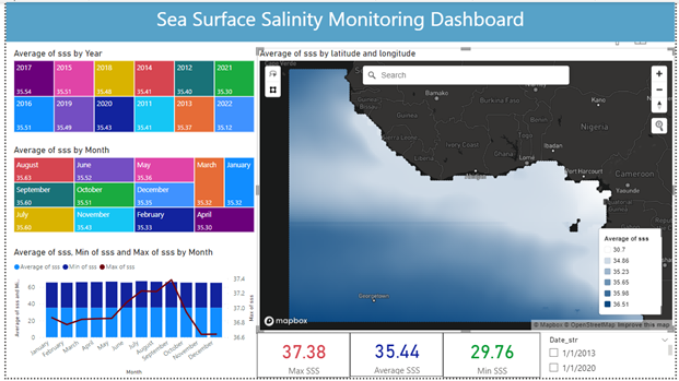
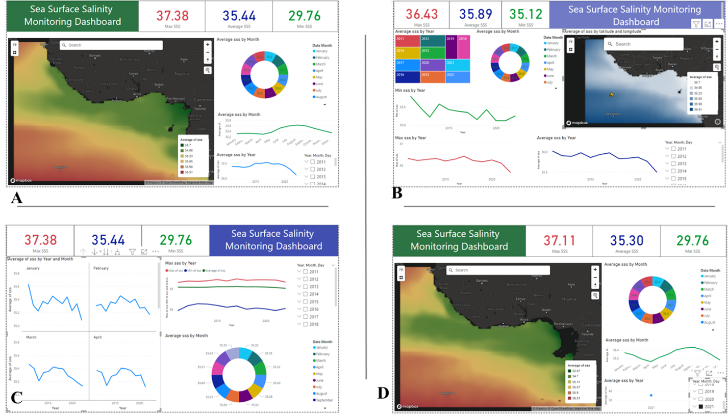
PowerBI tool was used to develop an interactive reporting dashboard to enable users to interact with the generated datasets (Fig. 2). Relevant visual widgets and charts were used to develop the various interfaces. This will enable the public, especially non-remote sensing experts to visualize and interact with the results generated in this research. The dashboard shows the key statistics of the SSS values in the study area, in addition to maps and graphs showing the annual, monthly, and weekly variations in the SSS values. In addition, users can drill down to individual data points and investigate the values across various timescales.
The combination of the End-to-End Extract ETL tool (developed with Python) with the Power BI-based reporting dashboard yielded the ETLAR tool.
5 Results
In this research we found that generally, SSS values varied spatially and temporally across the study area and period. Lower salinity values are recorded closer to the coasts. This is especially noticeable around the eastern flanks of the study area around the coasts of Nigeria (River Niger estuary), Cameroon (Rey Estuary), Equatorial Guinea (mouth of Rio Muni), Gabon (Gabon Estuary), and Angola (mouth of River Congo), which contain the mouth of major rivers in the respective countries (Fig. 3b). Higher SSS values were recorded farther into the Southern Atlantic Ocean.
Results obtained from this study shows that Sea surface salinity (SSS) within the study area were slightly less than 38 psu. Overall, average SSS of 35.41 psu was observed for the study area, with maximum value of 37.38 psu recorded in September 2017 at a location (longitude: 10.125, latitude: -8.625) off the coast of Luanda, Angola, and minimum value of 29.75 psu recorded in December 2021 at location (longitude: 5.625, latitude: 3.875) off the coast of Brass in the Bight of Biafra, Nigeria.
Fig. 3a shows the statistical trend of the annual minimum values. Maximum minimum value of 36.378 was recorded in 2018 at location (longitude: -22.375, latitude: -9.875) deep inside the South Atlantic Ocean between continental Africa and South America. Minimum minimum value of 29.749 was recorded in 2020 at a location (longitude: 6.375, latitude: 3.875) off the Bight of Biafra, off the coast of Nigeria.
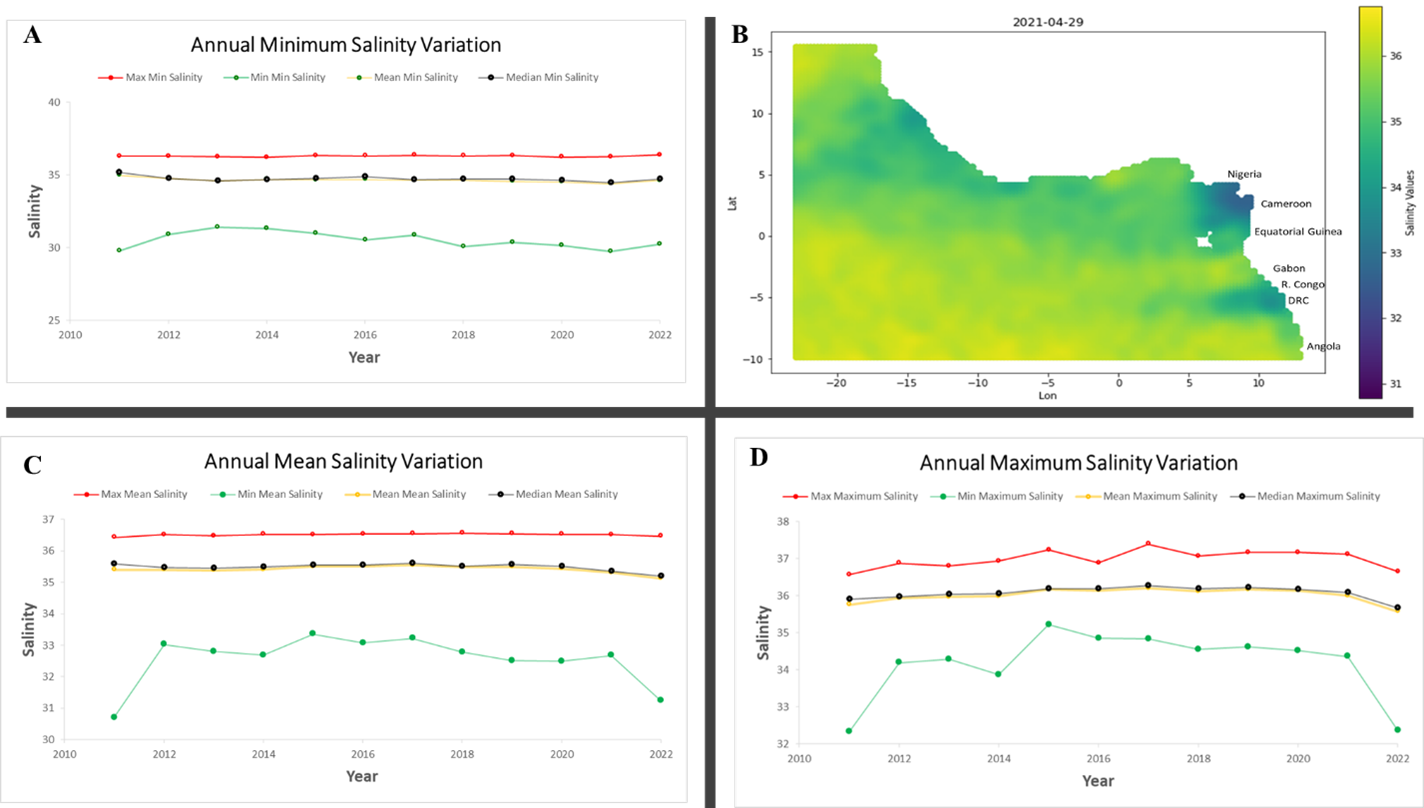
The statistical trends obtained from the annual mean values are shown in Fig. 3c. Mean average annual value of 35.43 psu was observed. Maximum average annual value of 36.562 was recorded in 2018 at a location (longitude: -21.875, latitude: -9.875) deep inside the South Atlantic Ocean between continental Africa and South America. Minimum average value of 30.698 was recorded in 2011 at location (longitude: 9.625, latitude: 2.875) off the coast of Cameroon.
Fig. 3d shows the statistical trend observed for the maximum annual values. The year 2011 appeared to have lower SSS values compared to other years. However, this may be due to the fact that only partial data was collected for that year from August. Maximum maximum value of 37.384 was recorded in 2017 at location (longitude: 10.125, latitude: -8.625) off the coast of Luanda, Angola. Minimum maximum value of 32.327 was recorded in 2011 at location (longitude: 9.625, latitude: 3.125) off the coast of Cameroon.
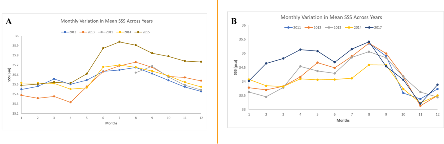
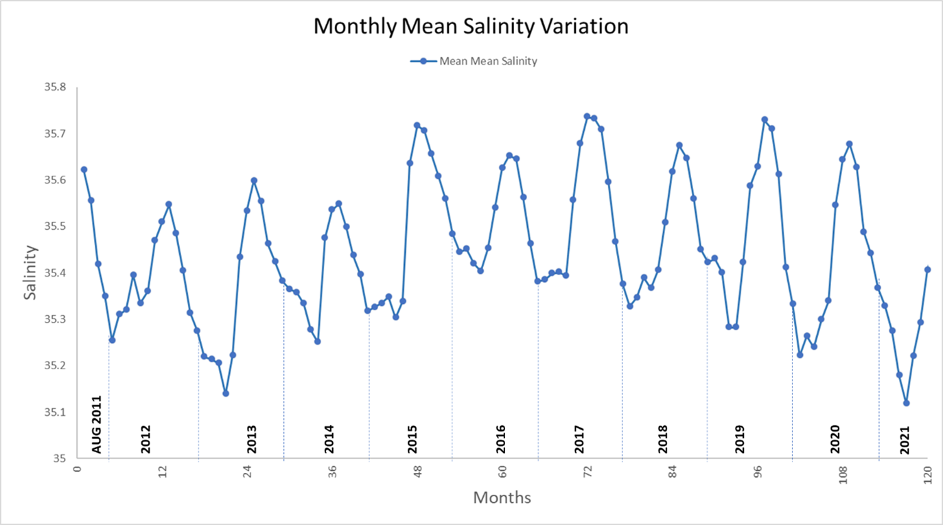
With respect to monthly aggregates of SSS, we observed that mean SSS across the study area tend to be highest between June and September with a peak in August, while lowest values are recorded in November/December (Fig. 4a).
This pattern was not only observed at the regional level (entire study area), locally, this pattern was also observed within the coast of Nigeria (Fig. 4b). Hence, suggesting that this pattern is consistent across the study area.
The longitudinal variation of the mean monthly salinity across the study period is shown in Fig. 5. This shows the sinusoidal variation of the SSS values across the months, year on year.
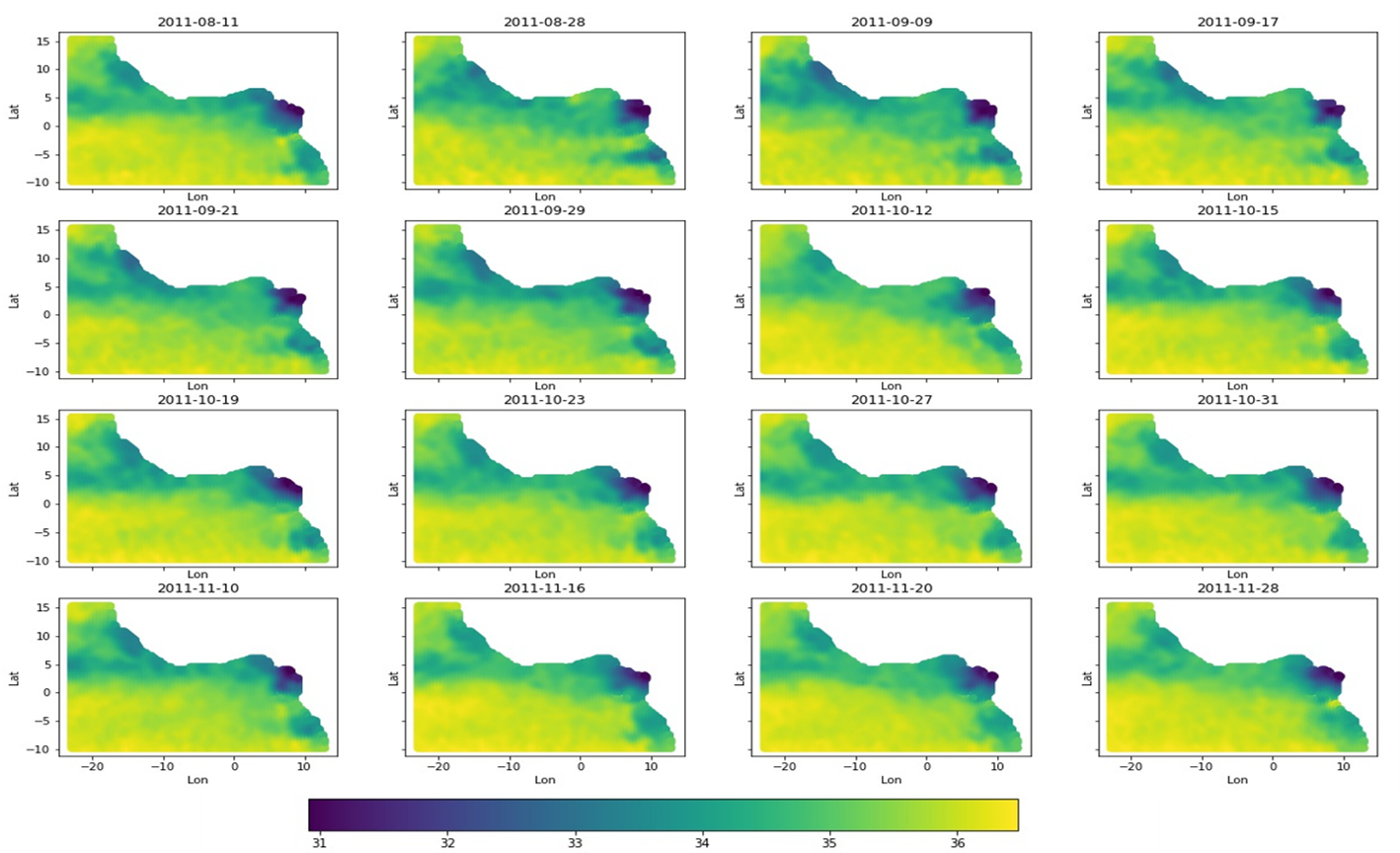
With respect to mapping of the SSS variations of individual data points, we developed the capability to map the variations in SSS at different aggregation levels (4-day), monthly, and annual. An illustration of the mapping of the sub-weekly (4 days) spatiotemporal variation in the salinity values of all data points in the study area is shown in Fig. 6.
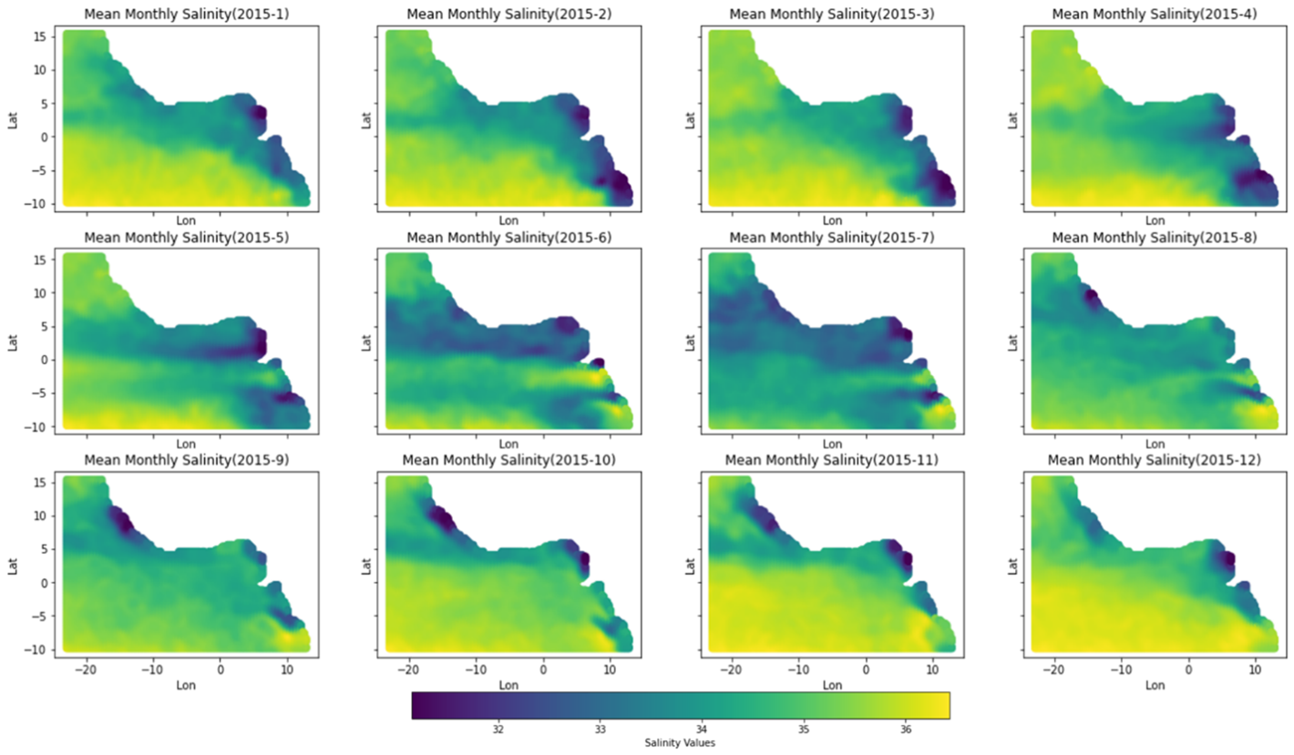
Time series maps of average monthly sea surface salinity of individual data points is shown in Fig. 7. Expectedly, inter monthly SSS variations observed here are noticeable compared to the intra monthly variations (Fig. 6). Lower SSS values were observed from May for September compared to the rest of the months. This contradicts the trend observed for the entire study area where the months of June to August were observed to have higher SSS values (Fig. 4).
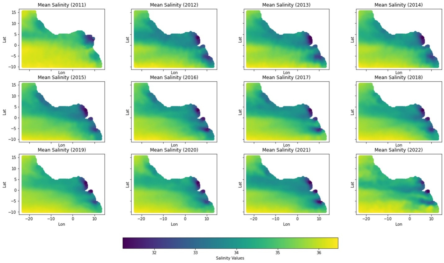
Spatiotemporal variation in annual mean salinity is shown in Fig. 8. The Fig. shows that the annual means recorded at each data point are fairly stable, without massive variation observed. The observation for 2011 and 2022 were observed to be slightly different and may have been skewed due to incomplete data.
Fig. 9 shows some pages from the interactive dashboard developed as part of this project. Key indicators shown are the maximum, average, and minimum SSS values. As an interactive dashboard, the values of these indicators can change depending on what options are selected by the dashboard user. By default, the values of the indicators are based on overall values for the entire study period. But users can drill down to a specific, year, month or weekly, for the entire study area or individual data point. For example, Fig. 9D shows the values derived for 2021 as against that of the entire study area shown in Fig. 9a. In the same vein, Fig. 9b shows averages from one data point, which can be selected by clicking on the map.
6 Discussion
In this research, we developed an automated method that can extract, process, and analyze sea surface salinity (SSS) data from the Optimally Interpolated Sea Surface Salinity (OISSS) dataset, a satellite product derived from the Aquarius and SMAP satellite missions. The technique developed has capability to process SSS values obtained from satellite data at various spatial scales (global, regional, national or for any specific location in the world) and temporal scale (sub-weekly, monthly, and annual).
Analysis of the SSS values extracted in this research revealed key trends in the variation of sea surface salinity in the study area across varying timescales. Key summaries of the trends were generated to enable quick understanding of the variations. A wide variance in salinity was observed for the study area with values ranging from a minimum of 29.749 psu to a maximum of 37.384 psu. This is due to the fact that the study area spanned through 5 latitudes and 8 latitudes, with varying influence of river inflow, evaporation rates and rainfall. The cold spots of salinity concentration were closer to the coasts especially those in the eastern flank of the study whereas the hot spots of SSS where towards the western flank of the study area towards the South Atlantic Ocean. The waters off the coast of Nigeria and Cameroon were found to be less saline than those of other countries within the study area, with an observed minimum SSS value of 29.749 psu, average salinity of 34.1 psu and maximum salinity of 35.8 psu. This reduced salinity is directly linked to the large river discharges (inflow) from the mouths of the major rivers in the area (River Niger and Rey River). Lower salinity values were also recorded closer to the coasts of other countries where major rivers flow into the ocean such as Equatorial Guinea (mouth of Rio Muni), Gabon (Gabon Estuary), Angola (mouth of River Congo), Senegal (River Casamance), The Gambia (River Gambie), and Guinea-Bissau (Rio Geba; Fig. 3).
Noticeable variations in the annual maximum and minimum values were observed, however, it was found that in general, annual mean salinity variation in the study area is fairly stable, with not much noticeable variation year-on-year. Although, a slightly higher annual mean value was observed in 2017. This relatively stable annual means observed at each data point indicate that the dynamic forces acting within the study are stable (in equilibrium; Fig. 8). Despite the stability observed in the annual means, intra-annual (monthly) variations were observed, with certain months of the year having higher salinity than others, due to interplay between the various key drivers of salinity (e.g. rainfall, inflow from rivers, and evaporation). However, this intra-annual variation were also found to be stable year on year, suggesting a stable pattern of variation.
The relatively high spatial resolution of the data used in this research, provides the capability for research to have detailed understanding of variations in sea surface salinity. The data points used in generating the SSS values are spread over a 0.25-degree grid. Hence, providing the capability to map the spatio-temporal variations of individual datapoints at approximately 28 km interval. The 28 km spatial resolution of data is quite useful as it enabled the understanding of variations SSS for a specific point or across a wider area of interest. This is very relevant considering that it would have been practically impossible to achieve this level of precision on a continuous basis, using traditional methods such as those used in deriving the underlying data used in the Copernicus Marine Service. Furthermore, continuous coverage of SSS can be derived from the discrete values recorded at the data points, by deploying spatial interpolation methods. In addition, further aggregations can be made from these individual values to regional or global summaries, which can provide useful insights to the patterns of variation and associated impacts on regional climatic conditions. This enhanced flexibility in data analysis and visualization incorporated in this research gives this an edge over existing marine visualization services such as the Copernicus Marine currently in existence, which somewhat have some rigidity in the user interactivity with the interface. In addition, this work also differs from the products of the Copernicus Marine due to the fact that the data used in the Copernicus Marine are produced from statistical models based on data obtained from global networks of different types of instruments: Argo floats (Argo1, OceanSites2, GOSUD3, EGO4, ITP), Meteorological data exchange network (Global Telecommunication System, GTS), conductivity-temperature-depth profiler (CTD), expendable bathythermograph (XBT) and expendable conductivity-temperature-depth profiler (XCTD), moorings, drifting buoys and sea mammals (Szekely, 2022; Copernicus Marine Service, 2023).
The monthly SSS variation observed across individual data points with decreased SSS around the months May, June, July, August, and September (Fig. 7) is particularly interesting as those months coincides with the peak of the rainy season in most of parts of the study area. This suggests that the inflow of runoff water into the sea from various estuaries dotting the study area, exerts some level of impact on the salinity levels in the ocean. However, whereas the monthly variations at individual data points showed decreased SSS values from May to September (Fig. 7), mean monthly values computed with all data points across the study area, showed that the months of June to August generally, had higher SSS values (Fig. 4). These apparent contradictory trends stem from the fact that the study area spanned through a diverse range of latitude (-10° to 15°) and longitude (-23° to 13°) as shown in Fig. 1. Both trends are useful in understanding the influence of SSS on climate. Whereas the observations from the data points can be used to understand localized impacts, the trend obtained from the aggregated values might have more influence on regional and global climatic conditions, as it shows the trend pulled from all data points in the study area.
Significantly, the automated Extract Load Transform and Report (ETLAR) developed in this research will contribute in the democratization of remote sensing data (Lefebvre et al., 2021; Mariam, 2021). Hence, making it available for the wider research community and the public to access and use, without having to deploy complex remote sensing data processing. Sea Surface Salinity is an important ocean variable for understanding key ocean and climate processes (Jang et al., 2022). The Global Climate Observing System (GCOS) program has designated it as an Essential Climate Variable. Key components of water cycle evaporation (E) and precipitation (P) have been found to correlate with SSS (Durack, 2015; Lindstrom et al., 2015; Wüst, 1936). Hence, sea surface salinity patterns provide a reflection of the overlying patterns of evaporation and precipitation. This makes it possible to use SSS to infer atmospheric freshwater fluxes (E– P) at any given point in time. For instance, SSS could be deployed as an efficient global rain gauge (Schmitt, 2008). Furthermore. the interplay between sea surface salinity and temperature also contributes to the vertical flow through the thermohaline circulation that constitutes part of the large-scale ocean circulation (Dinnat et al., 2019) as well as acoustic velocities observed in estuaries (Anejionu & Ojinnaka, 2011). Therefore, the democratization of sea surface salinity data will stimulate wider interest in this area of study, as well as enabling the wider public to appreciate the importance of remote sensing in solving societal issues.
Furthermore, results obtained from this research make it possible for future trends of the SSS values to be predicted. Indeed, with the amount of data collected from the satellite data, machine learning techniques could be deployed to predict future SSS values and trends. Such predictions could play a vital role in modelling future climatic conditions in the region. With adequate computing resources, the automated scripts developed in this research can be deployed for global studies to present SSS data on a near-realtime basis (subject to data availability), as well as support global predictive analytics of future SSS values. The sea surface salinity data generated in this study can also be used alongside other relevant ocean dynamics data to investigate oceanic impacts on global climate change under varying conditions. Conversely, the ability to regularly monitor salinity in a consistent manner can lead to a better understanding of the effects of changing climate on salinity concentrations across the globe. It has been found that climatic changes have substantially amplified ocean salinity in the past 50 years (Chinese Academy of Sciences, 2023). According to the report, as the Earth is warming, the global water cycle amplifies, which subsequently affects the salinity concentrations.
This research has further highlighted the benefits of satellite-derived ocean salinity values. The traditional methods of measuring sea surface salinity observations (buoy networks, ships) which offer reliable datasets is costly and relatively slowly. Hence, making it impractical for covering large geographic areas on a regular basis. By using data derived from satellite data detailed analysis of the spatiotemporal variation in sea surface temperature has been determined. This is expected to play critical role in subsequent research that would be conducted in the study of the dynamics at play in the regional (across the coasts of Africa) and global waters. The processing of the extracted data and presentation in an interactive dashboard will enable active engagement of the scientific community and the general public with the data, thus aiding the maximization of the impact of the research. An ongoing work is developing a web interface that would enable the research community and the general public to easily access this data from the internet. The PowerBI used in developing the dashboard has inbuilt tools that facilitate web publishing of dashboards. We expect that the web interface will host information on other relevant ocean variables currently being derived from remote sensing satellites.
We encountered certain limitations in the course of this work. The first limitation was orchestrated by computing resources. Satellite data processing is a resource-intensive tasks and we have processed data from multiple years. To process global salinity data in a timely manner distributed computing resources, which could leverage on cloud computing technologies would be required. Due to this limitation, we were only able to process data from West and Central Africa.
Another limitation was the use of satellites in this project. Despite its numerous advantages, the accuracy of satellite-derived salinity cannot match those obtained from in-situ instruments (Bao et al., 2019). Hence, it has to be pointed out that, that the results obtained in this research may not be absolute. However, satellite data provides the capability for consistent, rapid, and general monitoring of salinity variations across the globe.
7 Conclusion
Sea surface salinity is an important ocean dynamic that contributes to oceanic and climatic condition. Due to its crucial role in ocean dynamic process, it can also be used to infer changes in the global climate. As with other ocean phenomenon, remote sensing systems have been developed to regularly obverse global sea surface salinity from space. Satellite remote sensing offers realistic solutions to such challenges encountered in acquiring and monitoring sea surface salinity on a regular basis. Salinity monitoring is necessitated by constant variability in salinity across the globe and its impact on local and global climatic regimes.
This research developed automated techniques for extracting and processing sea surface salinity data from relevant satellite data. The technique was used to extract available SSS data off the coast of West Africa, over an extended period (2011–2022). The data extracted from a satellite product provided useful insights into the SSS variations across various data points in the study area across weeks, months, and years. This is a key advantage of deployment of satellite sensors in monitoring sea surface conditions. Sea surface salinity values in the study area were found to be less that 38 psu within the period of study. The waters off the coast of Nigeria and Cameroon (River Niger estuary and Rey Estuary) appear to be less saline than those of other countries within the study area, with an observed minimum SSS value of 29.749 psu, average salinity of 34.1 psu and maximum salinity of 35.8 psu.
Significantly, the techniques developed in this research can be deployed/adapted to extract from other satellite data such as sea surface temperature, sea surface topography, sea winds, ocean waves and sea surface topography. This will lead to the democratization of satellite-derived data to non-remote sensing experts. Thus, the wider research community and the general publish could actively engage with the data, originally obtained from a satellite sensor.
References
Akhil, V. P., Lengaigne, M., Durand, F., Vialard, J., Chaitanya, A. V. S., Keerthi, M. G., Gopalakrishna, V. V., Boutin, J. and de Boyer Montégut, C. (2016). Assessment of seasonal and year-to-year surface salinity signals retrieved from SMOS and Aquarius missions in the Bay of Bengal. International Journal of Remote Sensing, 37(5), 1089–1114. https://doi.org/10.1080/01431161.2016.1145362
Anejionu, B. O. and Ojinnaka, O. (2011). Underwater Acoustics and Depth Uncertainties In the Tropics. The International Hydrographic Review. https://journals.lib.unb.ca/index.php/ihr/article/view/20874
Antonov, J. I. and Levitus, S. (2006). World ocean atlas 2005. Vol. 2: Salinity. NOAA Atlas NESDIS, 62.
Bao, S., Wang, H., Zhang, R., Yan, H. and Chen, J. (2019). Comparison of satellite-derived sea surface salinity products from SMOS, Aquarius, and SMAP. Journal of Geophysical Research: Oceans, 124, 1932–1944. https://doi.org/10.1029/2019JC014937.
Bell, M. J., Martin, M. J. and Nichols, N. K. (2004). Assimilation of data into an ocean model with systematic errors near the equator. Quarterly Journal of the Royal Meteorological Society, 130(598), 873–893. https://doi.org/10.1256/QJ.02.109
Bindoff, N. L., Cheung, W. W. L., Kairo, J. G., Arístegui, J., Guinder, V. A., Hallberg, R., Hilmi, N., Jiao, N. et al. (2019). Changing Ocean, Marine Ecosystems, and Dependent Communities. In H.-O. Pörtner, D. C. Roberts, V. Masson-Delmotte, P. Zhai, M. Tignor, E. Poloczanska, K. Mintenbeck, A. Alegría et al. (Eds.), IPCC Special Report on the Ocean and Cryosphere in a Changing Climate (pp. 447– 587). Cambridge University Press, Cambridge, UK and New York, NY, USA. https://doi. org/10.1017/9781009157964.007
Boutin, J., Chao, Y., Asher, W. E., Delcroix, T., Drucker, R., Drushka, K., Kolodziejczyk, N., Lee, T. et al. (2016). Satellite and in situ salinity understanding near-surface stratification and subfootprint variability. Bulletin of the American Meteorological Society, 97(8), 1391–1407. https://doi.org/10.1175/BAMS-D-15-00032.1
Boutin, J., Reul, N., Koehler, J., Martin, A., Catany, R., Guimbard, S., Rouffi, F., Vergely, J. L. et al. (2021). Satellite-Based Sea Surface Salinity Designed for Ocean and Climate Studies. Journal of Geophysical Research: Oceans, 126(11). https://doi.org/10.1029/2021JC017676
Brucker, L., Dinnat, E. P. and Koenig, L. S. (2014). Weekly gridded Aquarius L-band radiometer/scatterometer observations and salinity retrievals over the polar regions-Part 2: Initial product analysis. Cryosphere, 8(3), 915–930. https://doi.org/10.5194/ TC-8-915-2014
Burrage, D., Wesson, J. and Miller, J. (2008). Deriving sea surface salinity and density variations from satellite and aircraft microwave radiometer measurements: Application to coastal plumes using STARRS. IEEE Transactions on Geoscience and Remote Sensing, 46(3), 765–784. https://doi.org/10.1109/ TGRS.2007.915404
Carmack, E. C., Yamamoto-Kawai, M., Haine, T. W. N., Bacon, S., Bluhm, B. A., Lique, C., Melling, H., Polyakov, I. V. et al. (2016). Freshwater and its role in the Arctic Marine System: Sources, disposition, storage, export, and physical and biogeochemical consequences in the Arctic and global oceans. Journal of Geophysical Research: Biogeosciences, 121(3), 675–717. https:// doi.org/10.1002/2015JG003140
Copernicus Marine Service (2023). Global Ocean-Real time in-situ observations objective analysis. Global Ocean- Real time in-situ observations objective analysis | Copernicus Marine MyOcean Viewer (accessed 13 Aug. 2023).
Chinese Academy of Sciences (2023). Ocean salinity: Climate change is also changing the water cycle. https:// usys.ethz.ch/en/news-events/news/archive/2020/09/new-study-of-ocean-salinity-finds-substantial-amplifica-tion-of-the-global-water-cycle.html (accessed 12 Sep. 2023).
Curry, R., Dickson, B. and Yashayaev, I. (2003). A change in the freshwater balance of the Atlantic Ocean over the past four decades. Nature, 426(6968), 826–829. https://doi.org/10.1038/ nature02206
D’Addezio, J. M., Bingham, F. M. and Jacobs, G. A. (2019). Sea surface salinity subfootprint variability estimates from regional high-resolution model simulations. Remote Sensing of Environment, 233, 111365. https://doi.org/10.1016/J. RSE.2019.111365
Droppleman, J. D., Mennella, R. A., Evans, D. E., Droppleman, J. D., Mennella, R. A. and Evans, D. E. (1970). An airborne measurement of the salinity variations of the Mississippi River Outflow. JGR, 75(30), 5909–5913. https://doi.org/10.1029/ JC075I030P05909
Durack, P. J., Wijffels, S. E. and Matear, R. J. (2012). Ocean salinities reveal strong global water cycle intensification during 1950 to 2000. Science, 336(6080), 455–458. https://doi.org/10.1126/science.1212222
Fine, R. A., Willey, D. A. and Millero, F. J. (2017). Global variability and changes in ocean total alkalinity from Aquarius satellite data. Geophysical Research Letters, 44(1), 261–267. https://doi.org/10.1002/2016GL071712
Fournier, S., Chapron, B., Salisbury, J., Vandemark, D. and Reul, N. (2015). Comparison of spaceborne measurements of sea surface salinity and colored detrital matter in the Amazon plume. Journal of Geophysical Research: Oceans, 120(5), 3177–3192. https://doi.org/10.1002/2014JC010109
Gierach, M. M., Vazquez-Cuervo, J., Lee, T. and Tsontos, V. M. (2013). Aquarius and SMOS detect effects of an extreme Mississippi River flooding event in the Gulf of Mexico. Geophysical Research Letters, 40(19), 5188–5193. https://doi.org/10.1002/ GRL.50995
Glenn, S., Schofield, O., Dickey, T. D., Chant, R., Kohut, J., Barrier, H., Bosch, J., Bowers, L. et al. (2004). The expanding role of ocean color and optics in the changing field of operational oceanography. Oceanography, 17(SPL.ISS. 2), 86–95. https:// doi.org/10.5670/OCEANOG.2004.52
Good, S. A., Martin, M. J. and Rayner, N. A. (2013). EN4: Quality controlled ocean temperature and salinity profiles and monthly objective analyses with uncertainty estimates. Journal of Geophysical Research: Oceans, 118(12), 6704–6716. https://doi. org/10.1002/2013JC009067
Grodsky, S. A., Kudryavtsev, V. N., Bentamy, A., Carton, J. A. and Chapron, B. (2012). Haline hurricane wake in the Amazon/Orinoco plume: a QUARIUS/SACD and SMOS observations. Geophys Res Lett, 39(12), L20603. https://doi. org/10.1029/2012gl052091
IPCC (2018). The Intergovernmental Panel on Climate Change: Summary for Policymakers. In V. Masson-Delmotte, P. Zhai, H. O. Pörtner, D. Roberts, J. Skea, P. R. Shukla et al. (Eds.), Global warming of 1.5°C. An IPCC Special Report on the impacts of global warming of 1.5°C above pre-industrial level (p. 32).
Jang, E., Kim, Y. J., Im, J., Park, Y. G. and Sung, T. (2022). Global sea surface salinity via the synergistic use of SMAP satellite and HYCOM data based on machine learning. Remote Sensing of Environment, 273, 112980. https://doi.org/10.1016/J. RSE.2022.112980
Korosov, A., Counillon, F. and Johannessen, J. A. (2015a). Monitoring the spreading of the Amazon freshwater plume by MODIS, SMOS, Aquarius, and TOPAZ. Journal of Geophysical Research: Oceans, 120(1), 268–283. https://doi.org/10.1002/2014JC010155
Korosov, A., Counillon, F. and Johannessen, J. A. (2015b). Monitoring the spreading of the Amazon freshwater plume by MODIS, SMOS, Aquarius, and TOPAZ. Journal of Geophysical Research: Oceans, 120(1), 268–283. https://doi.org/10.1002/2014JC010155
Lagerloef, G. (2012). Satellite mission monitors Ocean surface Salinity. Eos Trans AGU, 93(25), 233. https://doi. org/10.1029/2012eo250001
Land, P. E., Findlay, H. S., Shutler, J. D., Ashton, I. G. C., Holding, T., Grouazel, A., Girard-Ardhuin, F., Reul, N. et al. (2019). Optimum satellite remote sensing of the marine carbonate system using empirical algorithms in the global ocean, the Greater Caribbean, the Amazon Plume and the Bay of Bengal. Remote Sensing of Environment, 235, 111469. https://doi. org/10.1016/j.rse.2019.111469
Land, P. E., Shutler, J. D., Findlay, H. S., Girard-Ardhuin, F., Sabia, R., Reul, N., Piolle, J. F., Chapron, B. et al. (2015). Salinity from space unlocks satellite-based assessment of ocean acidification. Environmental Science & Technology, 49(4), 1987–1994. https://doi.org/10.1021/ES504849S
Lee, T., Lagerloef, G., Gierach, M. M., Kao, H. Y., Yueh, S. and Dohan, K. (2012). Aquarius reveals salinity structure of tropical instability waves. Geophysical Research Letters, 39(12). https://doi.org/10.1029/2012GL052232
Lefebvre, H., Legner, C. and Fadler, M. (2021). Data democratization: toward a deeper understanding. Forty-Second International Conference on Information Systems (ICIS), 1–17.
Lind, S., Ingvaldsen, R. B. and Furevik, T. (2018). Arctic warming hotspot in the northern Barents Sea linked to declining seaice import. Nature Climate Change 2018 8:7, 8(7), 634–639. https://doi.org/10.1038/s41558-018-0205-y
Mariam, C. (2021). Barriers to Democratising Space Data for Global Business | 4EI. https://www.4earthintelligence.com/ insights/barriers-to-democratising-space-data-for-global-business (accessed 12 Sep. 2023).
Melzer, B. A. and Subrahmanyam, B. (2015). Investigating decadal changes in sea surface salinity in oceanic subtropical gyres. Geophysical Research Letters, 42(18), 7631–7638. https://doi.org/10.1002/2015GL065636
NASA. (2022). NASA Salinity: Overview. https://salinity.oceansciences.org/overview.htm (accessed 12 Sep. 2023).
Palmer, M. D., Durack, P., Chidichimo, M. P., Church, J., Cravatte, S. E., Hill, K. L., Johannessen, J., Karstensen, J. et al. (2019). Adequacy of the ocean observation system for quantifying regional heat and freshwater storage and change. Frontiers in Marine Science, 6. https://doi.org/10.3389/FMARS.2019.00416
Pradesh, A. (2019). Ocean: Physical, Chemical, And Biological Characteristics. https://unacademy.com/content/kerala-psc/study-material/geography/ocean (accessed 12 Sep. 2023).
Qu, T., Song, Y. T. and Maes, C. (2014). Sea surface salinity and barrier layer variability in the equatorial Pacific as seen from Aquarius and Argo. Journal of Geophysical Research: Oceans, 119(1), 15–29. https://doi.org/10.1002/2013JC009375
Rani, M., Masroor, M. and Kumar, P. (2021). Remote sensing of Ocean and Coastal Environment – Overview. Remote Sensing of Ocean and Coastal Environments, 1–15. https://doi.org/10.1016/B978-0-12-819604-5.00001-9
Reul, N., Grodsky, S. A., Arias, M., Boutin, J., Catany, R., Chapron, B., D’Amico, F., Dinnat, E. et al. (2020). Sea surface salinity estimates from spaceborne L-band radiometers: An overview of the first decade of observation (2010–2019). Remote Sensing of Environment, 242, 111769. https://doi.org/10.1016/J. RSE.2020.111769
Reul, Nicolas, Quilfen, Y., Chapron, B., Fournier, S., Kudryavtsev, V. and Sabia, R. (2014). Multisensor observations of the Amazon-Orinoco river plume interactions with hurricanes. Journal of Geophysical Research: Oceans, 119(12), 8271–8295. https:// doi.org/10.1002/2014JC010107
Roemmich, D., Jolla, J., Boebel, O., Desaubies, Y., Freeland, H., King, B., LeTraon, P.-Y., Molinari, R. et al. (1999). Argo: The global array of profiling floats. Newsletter of the Climate Variability and Predictability Programme (CLIVAR), 4(3). https://oceanrep.geomar.de/id/eprint/7788/1/Exchanges13.pdf (accessed 12 Sep. 2023).
Schroeder, T., Devlin, M. J., Brando, V. E., Dekker, A. G., Brodie, J. E., Clementson, L. A. and McKinna, L. (2012). Inter-annual variability of wet season freshwater plume extent into the Great Barrier Reef lagoon based on satellite coastal ocean colour observations. Marine Pollution Bulletin, 65(4–9), 210–223. https://doi.org/10.1016/j.marpolbul.2012.02.022
Siedler, G., Church, J., Gould, J. (Eds. . (2001). Ocean Circulation and Climate: Observing and Modelling the Global Ocean. In Academic Press, London.
Skliris, N., Marsh, R., Josey, S. A., Good, S. A., Liu, C. and Allan, R. P. (2014). Salinity changes in the World Ocean since 1950 in relation to changing surface freshwater fluxes. Climate Dynamics 2014 43:3, 43(3), 709–736. https://doi.org/10.1007/ S00382-014-2131-7.
Smyth, K. and Mike E. (2016). Effects of changing salinity on the ecology of the marine environment. In M. Solan and N. Whiteley (Eds.), Stressors in the Marine Environment: Physiological and ecological responses; societal implications. Oxford Academic. https://doi.org/10.1093/acprof:oso/9780198718826.003.0009
Stammer, D., Martins, M. S., Köhler, J. and Köhl, A. (2021). How well do we know ocean salinity and its changes? Progress in Oceanography, 190, 102478. https://doi.org/10.1016/J. POCEAN.2020.102478
Stammer, D., Bracco, A., Achutarao, K., Beal, L., Bindoff, N., Braconnot, P., Cai, W., Chen, D. et al. (2019). Ocean climate observing requirements in support of climate research and climate information. Frontiers in Marine Science, 6. https://doi. org/10.3389/FMARS.2019.00444
Supply, A., Boutin, J., Vergely, J. L., Kolodziejczyk, N., Reverdin, G., Reul, N. and Tarasenko, A. (2020). New insights into SMOS sea surface salinity retrievals in the Arctic Ocean. Remote Sensing of Environment, 249, 112027. https://doi.org/10.1016/J. RSE.2020.112027
Szekely, T. (2022). In Situ TAC objective analysis Products. Product user manual. European Commission. https://catalogue.marine.copernicus.eu/documents/PUM/CMEMS-INSPUM-013-002-052.pdf (accessed 12 Sep. 2023).
Boyer, T. P. and Levitus, S. (2002). Harmonic analysis of climatological sea surface salinity. J Geophys Res, 107(C12), 8006.
Vinogradova, N., Lee, T., Boutin, J., Drushka, K., Fournier, S., Sabia, R., Stammer, D., Bayler, E. et al. (2019). Satellite Salinity Observing System: Recent Discoveries and the Way Forward. Frontiers in Marine Science, 6. https://doi.org/10.3389/ FMARS.2019.00243
Wang, S., Wang, C., Zhang, C., Xue, J., Wang, P., Wang, X., Wang, W., Zhang, X. et al. (2022). A classification-based spatiotemporal adaptive fusion model for the evaluation of remotely sensed evapotranspiration in heterogeneous irrigated agricultural area. Remote Sensing of Environment, 273. https://doi. org/10.1016/j.rse.2022.112962
Weller, R. A., Baker, D. J., Glackin, M. M., Roberts, S. J., Schmitt, R. W., Twigg, E. S. and Vimont, D. J. (2019). The challenge of sustaining ocean observations. Frontiers in Marine Science, 6(MAR). https://doi.org/10.3389/FMARS.2019.00105
Zweng, M. M., Reagan, J. R., Seidov, D., Boyer, T. P., Locarnini, R. A., Garcia, H. E., Mishonov, A. V., Baranova, O. K. et al. (2018). World Ocean Atlas 2018, Volume 2: Salinity. In A. Mishonov (Technical Ed.), NOAA Atlas NESDIS, 82.
Authors’ biographies

Dr. Obinna Anejionu is a lecturer at the Department of Geoinformatics and Surveying, University of Nigeria Nsukka. He obtained PhD in Geography (Remote Sensing and GIS) from Lancaster University, United Kingdom, M.Sc. in GIS wt. Remote Sensing from the University of Greenwich, London, United Kingdom, and M.Sc. in Hydrographic Surveying from the University of Nigeria Nsukka.
He has previously worked as a postdoc Research Associate at Imperial College London, and Spatial Data Scientist at the Urban Big Data Centre, University of Glasgow. His current research interests focus on deploying geospatial big data science, earth observation, and artificial intelligence to tackle relevant societal issues.

Dr. Elijah S. Ebinne is a Senior Lecturer at the Department of Geoinformatics and Surveying, University of Nigeria Nsukka. He has PhD in Geoinformatics and Remote Sensing, and M.Sc in Geodesy and Astronomy. His current research interests focuses on the remote sensing applications in aquatic environments and forestry.

Opeyemi Ajibola-James is a PhD student at the Department of Geoinformatics and Surveying, University of Nigeria Nsukka. He is also the CEO/MD/Data Scientist & Analyst/Researcher at Geo Inheritance Limited, Nigeria, where he plays a lead role in the development, management, and execution of the geospatial and non-spatial data services, which typically involve the integration of remotely sensed data with field observations, feature engineering, coding for data analyses, statistical and machine learning (ML) modelling and forecasting. He is a Fellow Member of Eudoxia Research University (FMERU), the USA, and a Fellow Member of Eudoxia Research Centre (FMERC), India.
Before joining Geo Inheritance Limited, he worked with the Shell Petroleum Development Company of Nigeria (SPDC) as a Research Attaché to Geomatics. He received B.Sc. (Hons.) in Geography and M.Sc. in Remote Sensing and GIS from the Obafemi Awolowo University, Nigeria. His current research interest focuses on integrated applications of Remote Sensing, GIS, Data Science, Data Analytics, and ML to provide interpretable, reliable, scalable, and affordable solutions that can support proactive and timely data-driven decisions in broad domains (Physical Oceanography, Climate Change, Geography, Environmental Pollution and Business Development).
- International profiling float network (www.argo.net, accessed 12 Sep. 2023) and its European component (https://www.euro-argo.eu, accessed 12 Sep. 2023).
- OceanSITES is a worldwide system of long-term, open-ocean reference stations (OceanSITES is a worldwide system of long-term, open-ocean reference stations ) and its European component (https://www.emso.eu, accessed 12 Sep. 2023).
- International Global Ocean Surface Underway Data (https://www.gosud.org, accessed 12 Sep. 2023).
- International Glider network (https://www.ego-network.org, accessed 12 Sep. 2023).