1 Introduction

GNSS instrumentation has been used for land surveying and geodetic positioning for more than thirty years. These communities rely on the use of carrier phase data, where multipath has long been known to be a source of error. In order to reduce the impact of multipath on positioning, multipath-suppressing antennas are almost always used. There have also been many efforts over the years to investigate different ways to remove multipath effects in carrier phase observables after the fact.

Here we examine a relatively new application for GNSS instruments known as GNSS interferometric reflectometry (GNSS-IR). This technique uses multipath rather than tries to remove it. This work is distinct from GNSS-R where reflected signals are observed in space using specialized receivers/antennas (Ruf et al., 2018). It is also distinct from ground- based GNSS reflection systems where the instruments have been modified to optimize the reflected GNSS signal (Anderson, 2000; Dunne et al., 2005; Löfgren & Haas, 2014). The goal of GNSS-IR is to measure the location and characteristics (i.e. its dielectric constant and roughness) of the surface below a GNSS antenna. In other words, the GNSS instrument is being used as a bi-static radar. Instead of the carrier phase data, the primary observable used in GNSS-IR is Signal to Noise Ratio (SNR) data. Generation of these SNR data requires no additional equipment as the measurements are generated by existing consumer-off the-shelf systems.

Although the GNSS-IR technique was first pioneered to measure soil moisture and snow accumulation (Larson et al., 2008; Larson et al., 2009), the focus of this paper is using GNSS-IR to measure water levels (Larson et al. 2013a; Löfgren et al., 2014; Larson et al., 2017). One of the advantages of using GNSS-IR for water level measurements is that the positioning information from GNSS can be combined to create a water level measurement defined in ITRF (Altamimi et al. 2023). In the next sections we will first describe the basic principles used in GNSS- IR and then introduce an open source software package, gnssrefl. The final section will present water level measurements from two representative sites using this new software.

2 Principles of GNSS-IR

2.1 Definition of multipath frequency

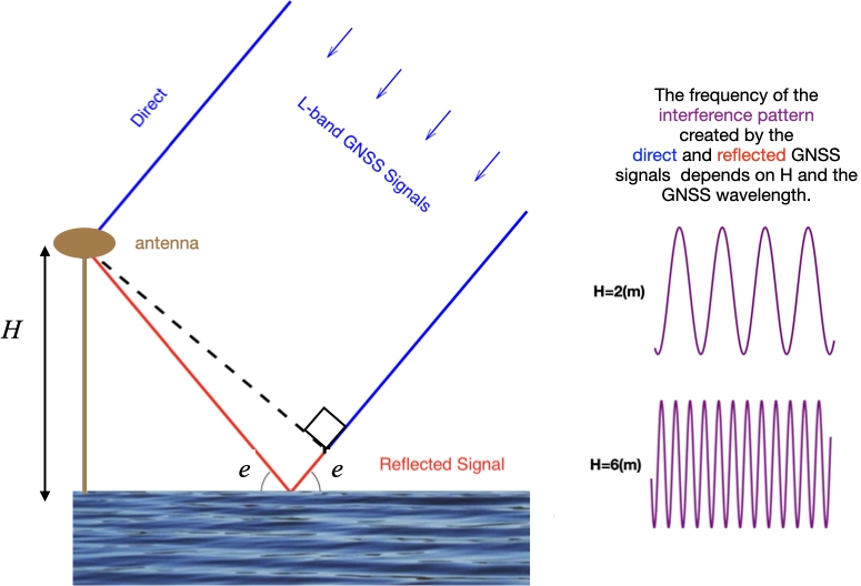
Multipath in GNSS observables is caused by GNSS signals that deviate from the direct path between the satellite transmitter and the receiving antenna. Although more complicated scenarios are possible, in Fig. 1 we present the simplest possible example of GNSS multipath, forward scatter from a horizontal planar surface below a GNSS antenna. The path of a representative direct signal is shown in blue, whereas the additional path taken by the reflected signal for the given geometry is shown in red.

The multipath frequency f in carrier phase observations caused by this horizontal planar reflection has been known for many years (Georgiadou & Kleusberg, 1988).

(1)

The elevation angle e is the angle of the GNSS satellite above the local horizon, H is the height of the antenna phase center above the reflecting surface (here termed the “reflector height”) and 𝜆 is the GNSS wavelength. If a GNSS antenna were surrounded by a large planar surface, in principle this multipath frequency could be determined from one of the GNSS observables and a correction profile for each satellite could be computed and applied (Bilich et al., 2008; Rost & Wanninger, 2009). In practice, very few GNSS instruments are operated in such simple surroundings and estimating the multipath frequency is difficult in real-world surroundings.

2.2 Observing multipath frequency

Multipath produces errors in both pseudorange and carrier phase GNSS data. Extracting the multipath frequency from those observations is challenging. Ideally one wants to be able to extract the frequency from an observable that can be clearly assigned to a specific reflecting surface. This can be done for individual pseudorange data arcs by using dual frequency phase data to remove geometric errors and the ionospheric effect; the data combination is in fact often called the multipath observable. Unfortunately, pseudorange data are particularly noisy at the low elevation angles where the multipath errors are most significant.

Carrier phase data are much more precise than pseudorange data, but there is no simple way to extract multipath errors from it. Multipath errors are clearly present in carrier phase post-fit residuals in positioning solutions, but these residuals are based on using all satellite observations at a given epoch. While one can assign multipath in those residuals to a specific surface based on the satellite number, it will always be at some level biased by the other satellite signals used in the positioning solution. Raw single frequency carrier phase observations can be differenced to remove the geometric effects, but these data combinations are degraded by both cycle slips and ionospheric effects (Ozeki & Heki, 2012).

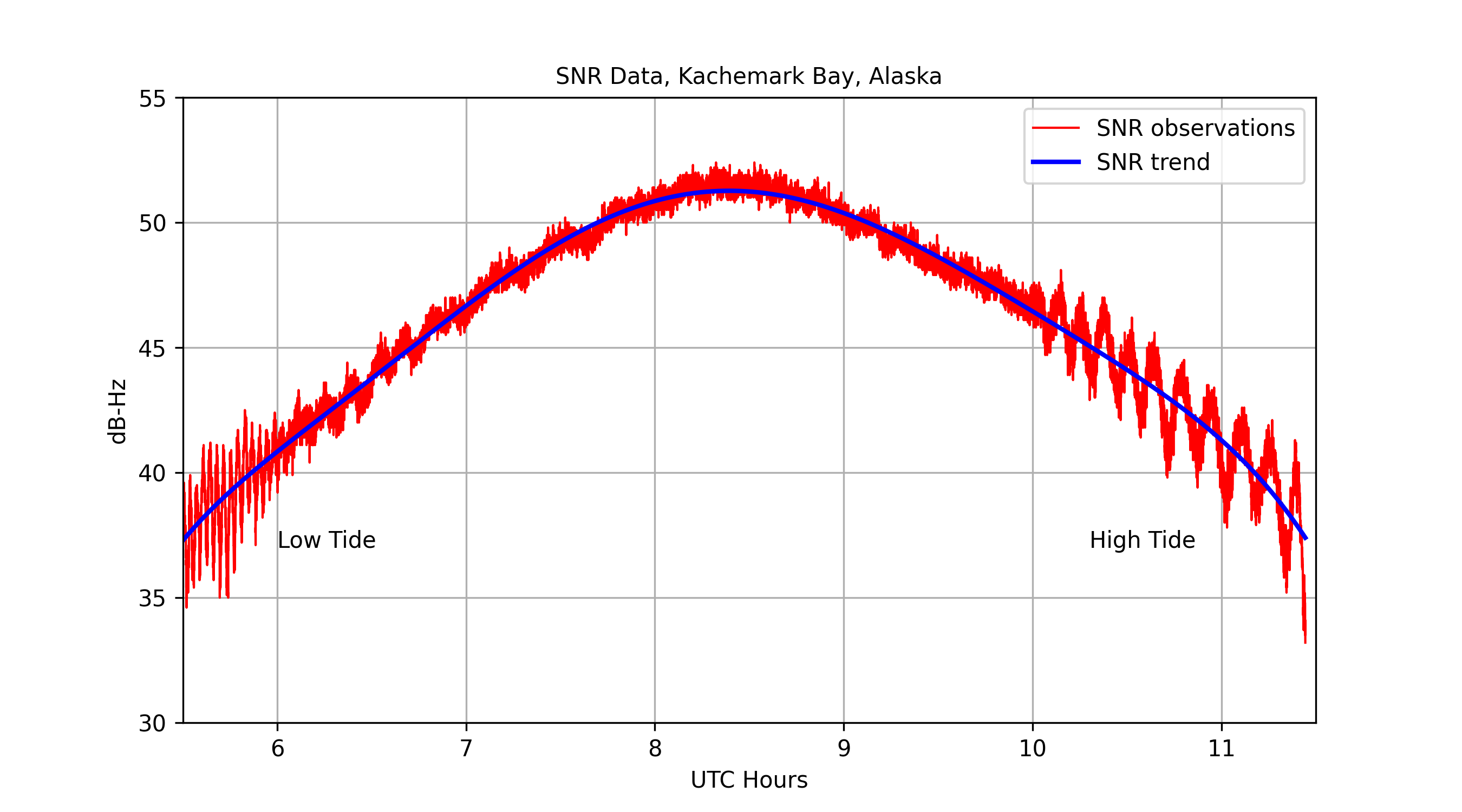
Because they tell you nothing about receiver positions, SNR data are generally ignored by surveyors and geodesists. However, SNR data are sensitive to multipath and thus are an alternative source of data for determining the multipath frequency. One advantage of using SNR data is that it has very simple background models. Fig. 2a shows representative SNR data for one satellite arc from a site in Alaska (Larson et al., 2013b). The smooth blue curve in the figure represents the direct signal or SNR trend, i.e. what the SNR data would look like if there were no multipath; the SNR trend can be generated from a simple polynomial fit. This contrasts with modeling carrier phase measurements, which requires precise models for the satellite/receiver positions, transmitter/antenna phase offsets, clocks, and atmospheric effects. The oscillations seen on the direct signal at the beginning and ending of the satellite arc are produced by water reflections. In this example the rising arc was coincident with low tide (high frequencies in the SNR data) and the setting arc was during high tide (low frequencies in the SNR data).

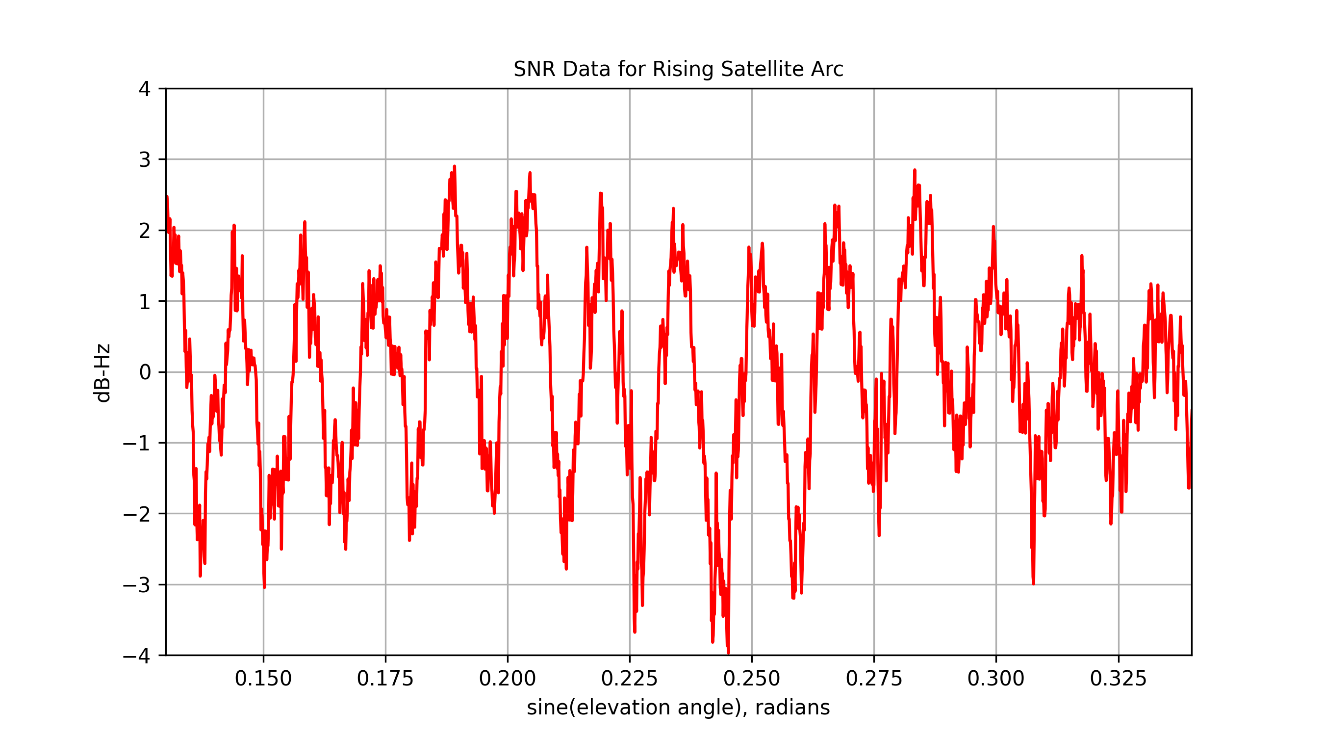
In order to estimate the multipath frequency from SNR data, Eq. 1 can be recast using sine of elevation angle rather than time or elevation angle (Axelrad et al., 2005). Once that SNR trend is removed (Fig. 2b), the SNR data for the rising and setting arcs can then be represented as:

(2)

Note that the multipath frequency 2H/𝜆 is now directly related to the reflector height H without the need for simultaneously modeling ė. The amplitude term A(e) is shown here to depend on elevation angle to make it clear that it is not a constant. It also depends on the roughness and dielectric constant of the reflecting surface and the antenna gain pattern. Any spectral technique that allows unevenly sampled data can then be used to estimate the multipath frequencies (and thus reflector height H) for the rising and setting data arcs that are needed to measure water surfaces. In gnssrefl a Lomb-Scargle periodogram is used to estimate H (Vanderplas, 2018).

3 Using GNSS-IR in practice

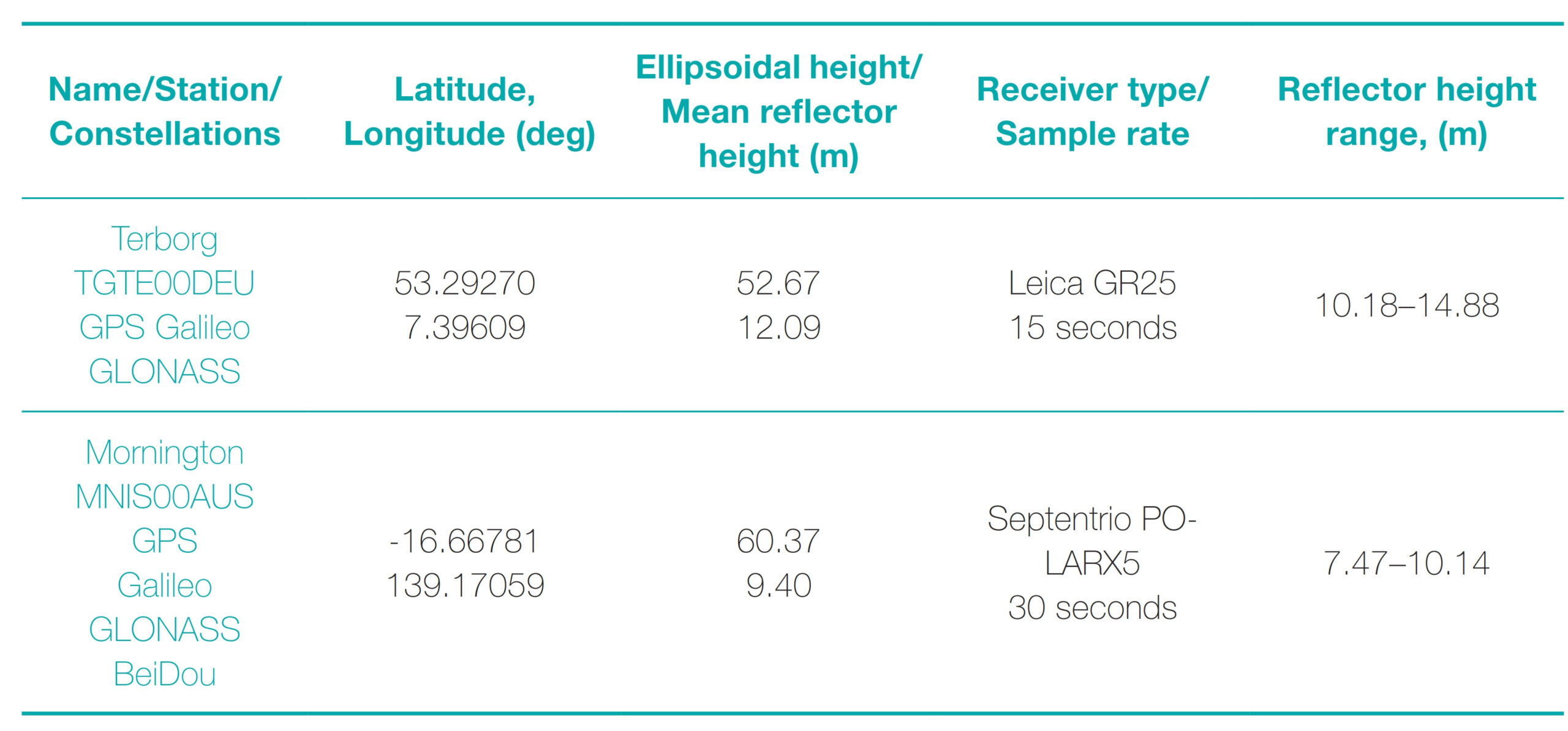
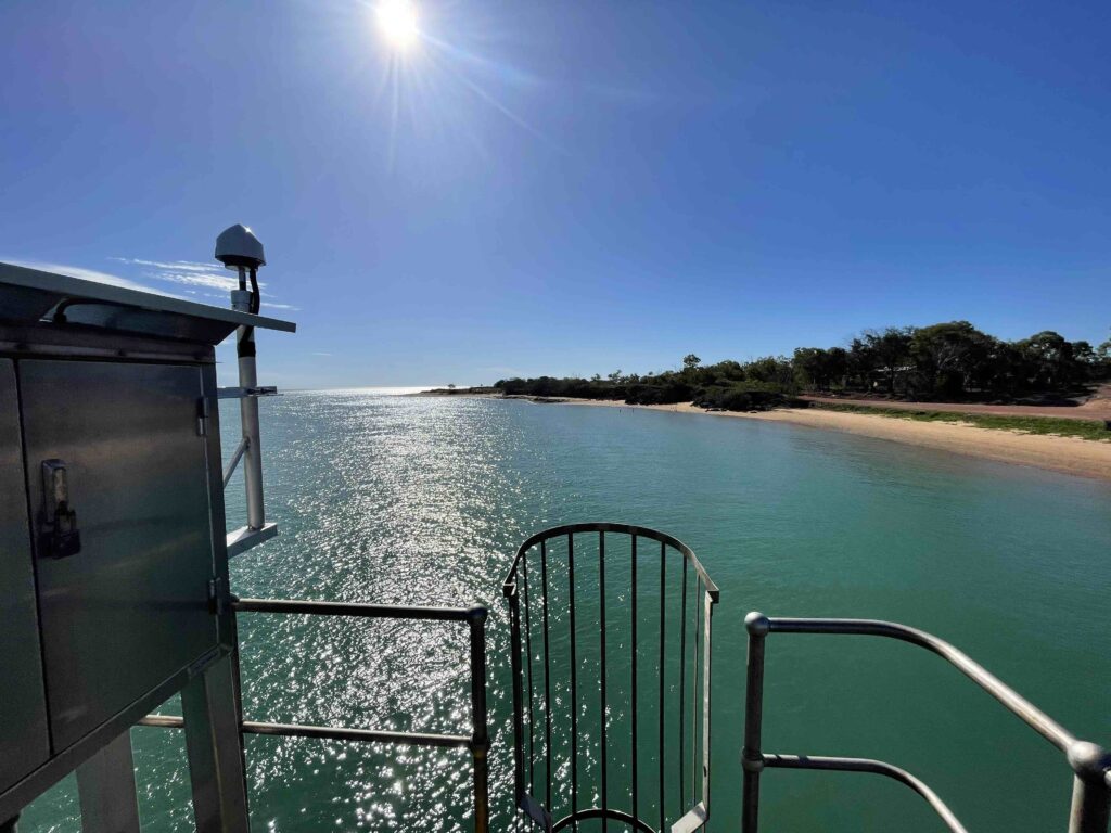
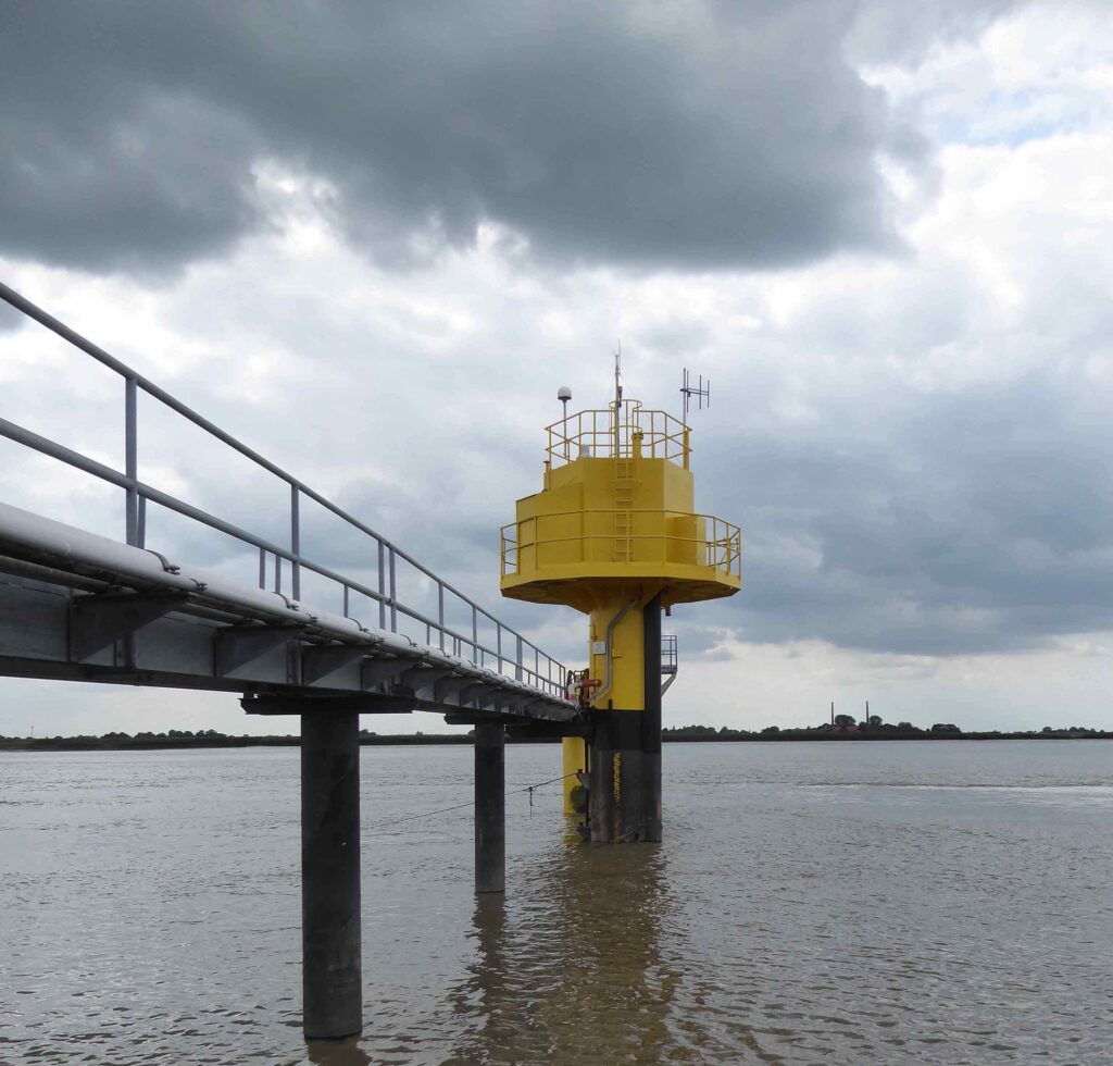
Sections 2.1 and 2.2 outline in principle how SNR data can be used to measure reflector heights at different times and thus be implemented to measure water levels. There are two additional steps that are needed before the GNSS-IR method can be used in practice. First, the user must ensure that the reflected signals come from the water. This is generally referred to as calculating the “station mask”. The second step is ensuring that the receiver sampling interval is sufficient to estimate the multipath frequency, and thus reflector height. Two GNSS stations will be used as examples: Mornington in Australia (Fig. 3a) and Terborg in Germany (Fig. 3b). Additional information about these GNSS stations is given in Table 1. These sites were chosen for the following reasons:

1. Both sites have collocated tide gauges which is useful here for validating the GNSS-IR water level measurements.
2. Each site tracks signals from at least three GNSS constellations and modern GPS signals (e.g. L2C, L5).

In each case the GNSS receivers are being operated for positioning and are not optimally located for GNSS-IR. The Terborg site, in particular, is likely impacted by ship traffic on the Ems river. It should also be noted that both these sites use a multipathsuppressing geodetic-quality antenna.

3.1 Reflection Zones

GNSS-IR requires that the antenna has a clear view of the reflection surface. For the most part the reflection area of the GNSS signals can be predicted by calculating the first Fresnel zones of each rising and setting satellite arc. These Fresnel zones depend on the reflector height H and the satellite’s elevation and azimuth angles. The equations for GNSS-IR Fresnel zones are given in the appendix of Larson & Nievinski (2013). gnssrefl allows users to project these Fresnel zones onto a Google Earth image. The user chooses:

1. Constellation (GPS, GLONASS, Galileo, or BeiDou)
2. Frequency (L1, L2, L5)
3. Azimuth angle limits
4. Elevation angle limits
5. Reflector height

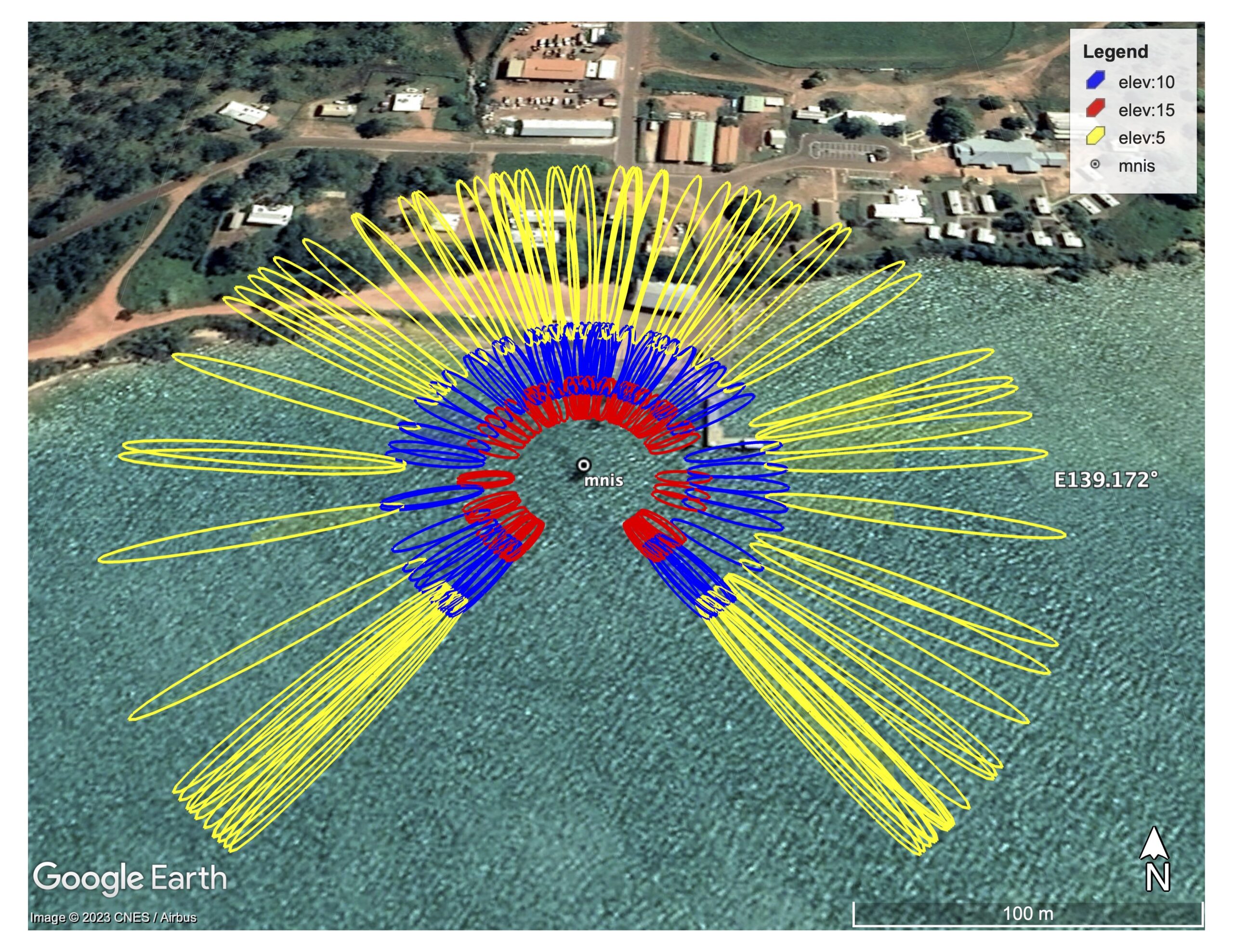
For water reflections, elevation angles of 5–15 degrees are generally ideal. Above 15 degrees the reflected signals from water surfaces are very small in amplitude; angles below 5 degrees are more susceptible to refraction error.

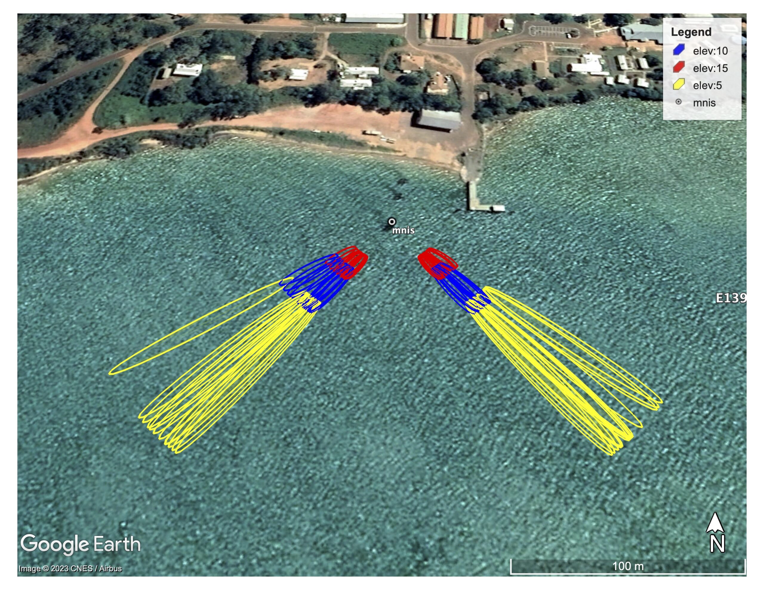
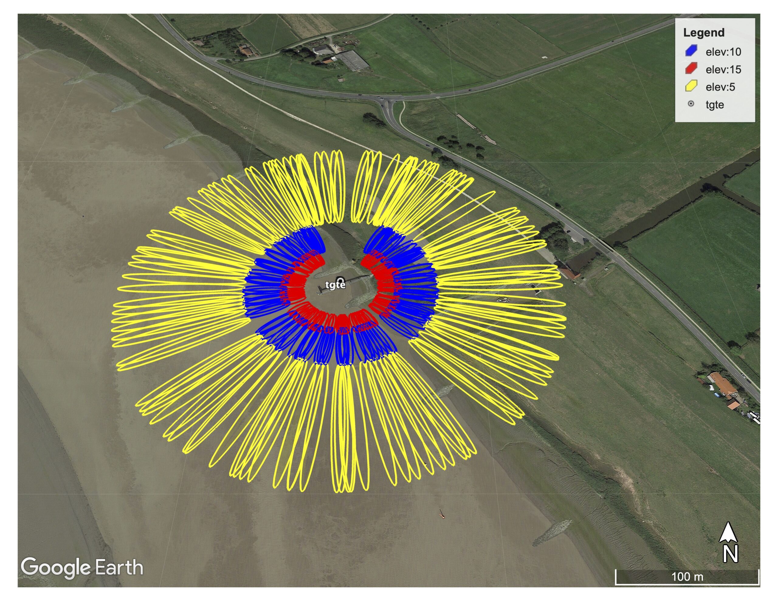
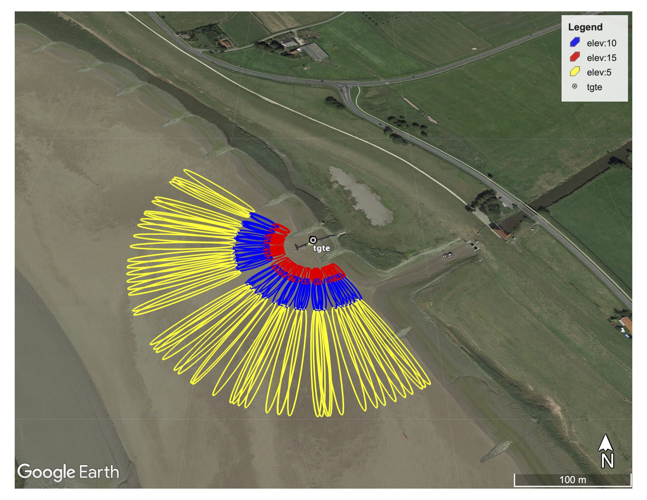
Fig. 4a shows the first Fresnel zones for GPS satellites on the L1 frequency at Mornington if all azimuths could be used. Each set of ellipses represents either a rising or setting satellite arc as would be observed at the antenna, which is located at the circle symbol. One can immediately see that the Mornington site is too close to the shore to use the rising and setting satellite tracks to the north. Some reflection zones will also be obstructed by a pier to the northeast. Most of the southern tracks, however, appear to be useable. Fig. 4b shows an edited azimuth mask for the site. Although the azimuth regions that can be used here are small in number, there is some compensation in that all four major GNSS constellations are tracked at this site.

Fig. 5a shows the first Fresnel zones for GPS satellites on the L1 frequency at Terborg. Clearly many of the reflections will be coming from the nearby riverbank and not the water. Fig. 5b is an edited mask that restricts azimuths to those that reflect off the Ems River. This mask should be considered as a first step, as there could still be obstacles at the site itself (trees, obstructions on the pier that hosts the GNSS antenna) that block reflected signals. Although many more satellite tracks can be viewed at Terborg than Mornington, only three constellations are tracked (GPS, GLONASS, and Galileo).

3.2 Maximum resolvable reflector height

In addition to setting an azimuth and elevation mask, GNSS-IR users must also evaluate the maximum resolvable reflector height for the prospective GNSS-IR site. This parameter is similar to the Nyquist frequency for a time series, but we recast the problem here in terms of reflector height. gnssrefl adopts the strategy of Roesler & Larson (2018) by calculating the maximum resolvable reflector height for each rising and setting satellite arc for a given constellation, frequency, reflector height, and receiver sampling interval.

The maximum resolvable reflector height varies by azimuth at a given GNSS site because the time derivative of elevation angle also varies by azimuth and station latitude. The calculated maximum resolvable reflector height values should be compared with the expected reflector heights at the site of interest. This calculation can be made before a GNSS unit is deployed as long as the user knows the approximate position of the GNSS site and has information about tidal variations in the region.

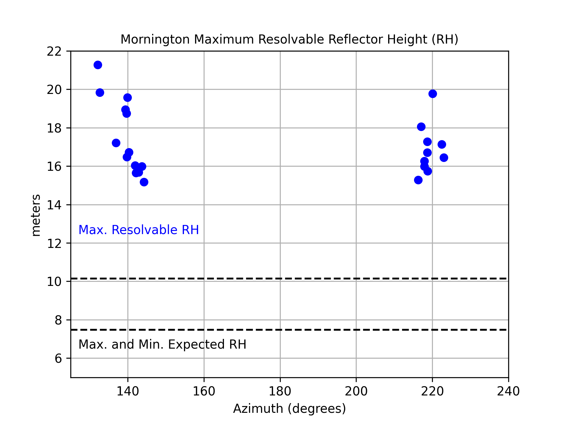
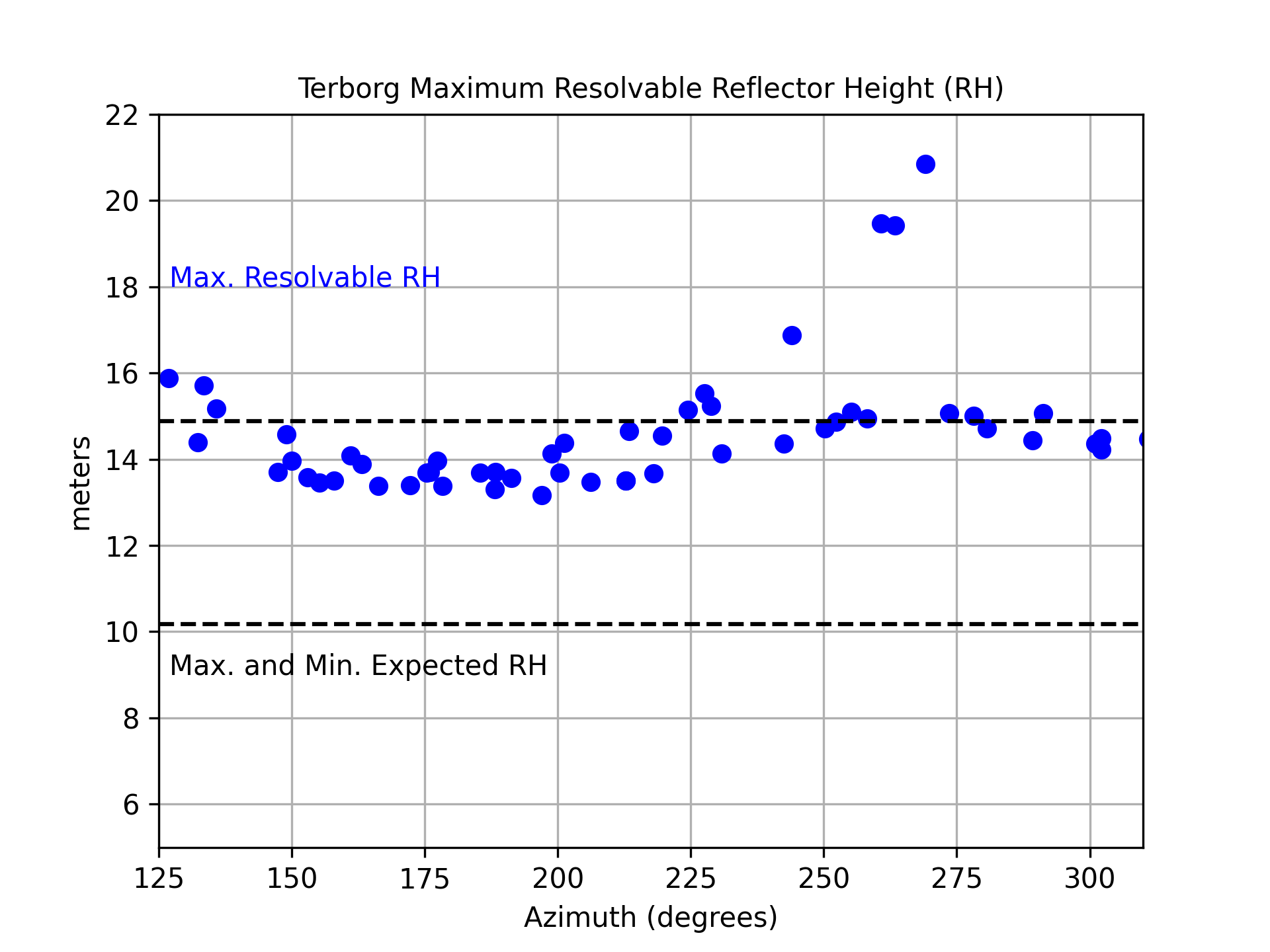
Fig. 6 shows the maximum resolvable reflector heights for Mornington and Terborg. In each case the L1 GPS frequency and 30 second receiver sampling is used for the calculation. At Mornington, the maximum resolvable reflector height varies from 15–20 meters. Based on longterm tidal records from the region, the water surface is expected to vary between reflector heights of 8–10 meters. This means that a 30 second receiver sampling interval is acceptable for Mornington. In contrast, almost half of the reflector heights from Terborg will be biased if 30 second sampling is used because the maximum resolvable reflector heights of 13–15 meters are too close to the expected reflector height limits. Operating the Terborg receiver at 15 seconds sampling instead of 30 seconds will shift the maximum resolvable reflector heights to 26–30 meters, which is far above the expected reflector height limits of 10–15 meters. The L2 and L5 GNSS wavelengths are larger than the L1 wavelength, and thus the maximum resolvable reflector heights for these frequencies will always be larger than the L1 values.

4 GNSS-IR: software and results

4.1 Open source software

GNSS-IR has been primarily developed by academic researchers using homegrown software. The water level measurements discussed in this section are based on gnssrefl, a GNSS-IR open source software package written in python (gnssrefl, 2023). Although originally envisioned for use by academic researchers with Linux computers, it can also be used on a PC by using docker containers (Docker, 2023). The latter obviates the need for users to install python on their local machines. Initially gnssrefl was limited to GNSS data saved in the Receiver Independent EXchange (RINEX) format, but it has been extended to allow National Marine Electronics Association (NMEA) records used by the realtime navigation community. gnssrefl can also be installed on a local machine by cloning the repository (gnssrefl, 2023) or using pypi (gnssrefl-pypi, 2023). Documentation for the package is provided at the GitHub repository in the self-documenting format frequently used in the python community.

gnssrefl can be used to analyze either personal GNSS datasets or archived GNSS datasets at international geodetic archives. More than a dozen GNSS archives are supported in gnssrefl. Once the GNSS SNR data have been translated into a tabular ASCII format, satellite azimuth and elevation angles are calculated using either GPS broadcast orbits or precise multi-GNSS orbits (GFZ-orbits, 2023). The tabular data files are then stored on a local machine.

The user must set a GNSS-IR analysis strategy, i.e. define the azimuth and elevation mask, the expected reflector height region, and various quality control parameters. Visualization tools are provided in gnssrefl to allow the user to confirm the validity of the requested azimuth and elevation mask. In the first step, reflector heights are estimated and quality control constraints are applied. A subsequent module is used to convert the reflector heights to water levels. For lakes, daily averages of the individual reflector heights are generally sufficient. For water bodies with significant subdaily variations from tides, gnssrefl also makes a correction for reflector height changes that occur during the rising or setting arc known as the Ḣ correction (Larson et al., 2013b) and removes interfrequency biases. Details about the software, along with examples for lakes, rivers, and the ocean are provided at the software repository (gnssrefl, 2023).

4.2 Web app

gnssrefl was developed so that users would have the most flexibility in finding GNSS data, orbits, generating reflector heights, and producing time series of water levels. A parallel initiative has led to the creation of a web application (gnssirapi, 2023). Examples of water levels analyzed with the GNSS-IR method are available with approximately 10 second latency. Users may also upload RINEX files to the site to generate reflector heights and evaluate reflection zones (Fresnel zones).

4.3 GNSS-IR Results

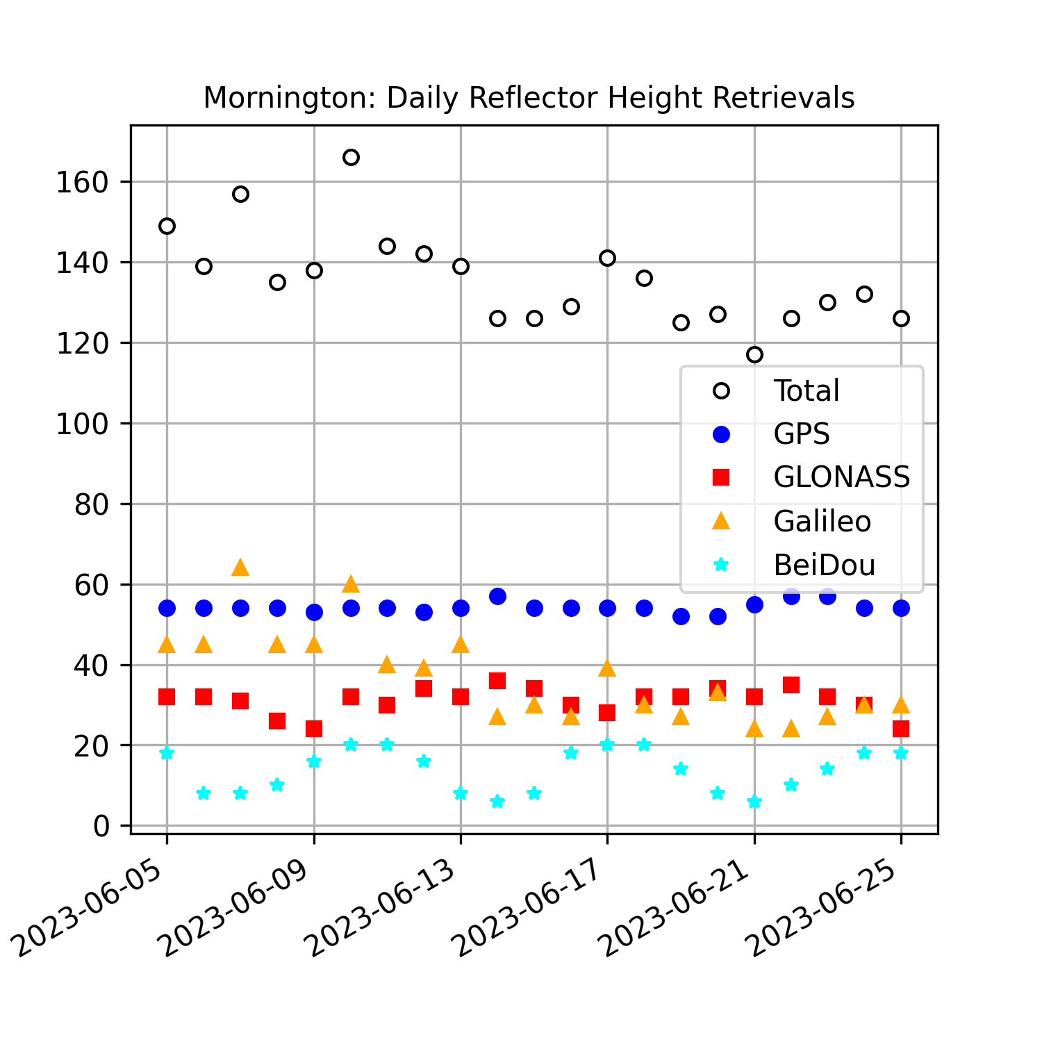
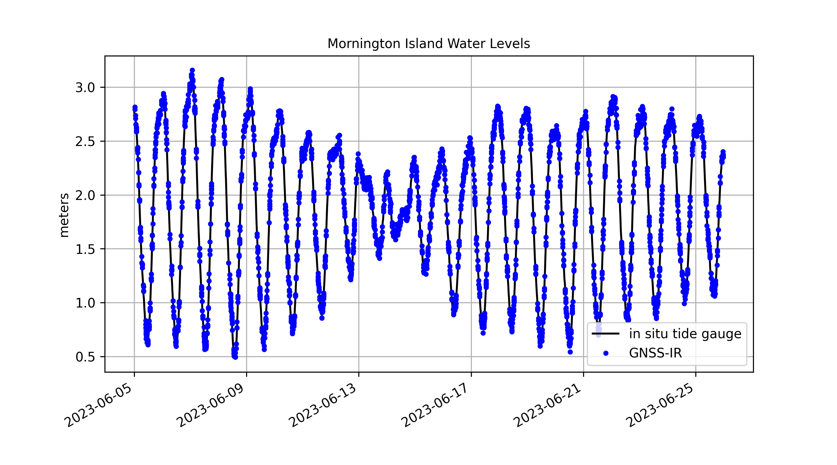
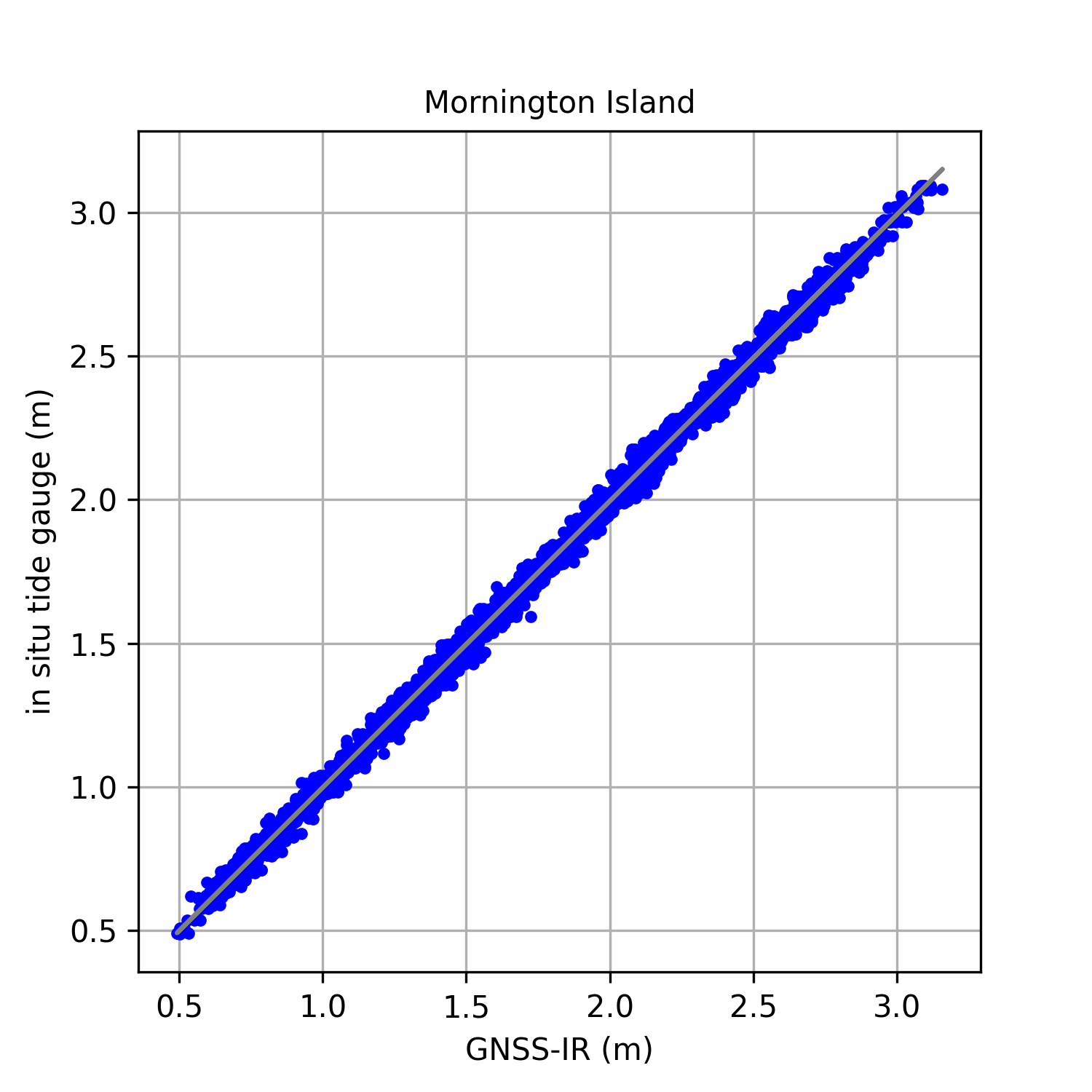
Fig. 7 summarizes the number of reflector height measurements that were estimated each day over a threeweek period at the Mornington site. The largest number of reflector height retrievals come from the GPS constellation while Beidou contributes the fewest. The temporal variation in retrievals for GLONASS, Galileo, and Beidou is due to these constellations having variable ground tracks, while GPS has a daily repeating ground track. To compare reflector heights with publicly available tide gauge data, we reverse the sign on the reflector height measurements and remove a bias from each dataset (Fig. 8). Although the agreement appears to be quite good, there are clearly temporal gaps in the GNSS-IR series. We can partially fill these temporal gaps by using smaller satellite arcs, thus producing more reflector heights per rising/setting satellite arc. However, the only other way to improve the temporal resolution of GNSS-IR for Mornington would be to place the GNSS antenna in a more optimal location. The correlation between the two series is 0.999 and the standard deviation of the residuals is 0.032 meters (Fig 9).

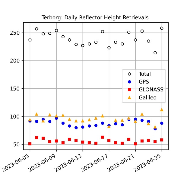
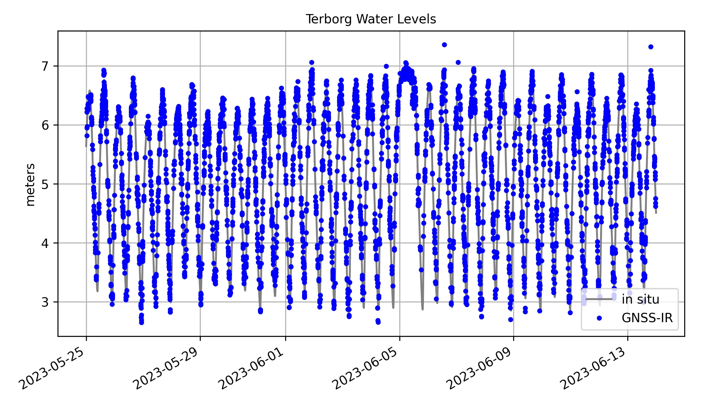
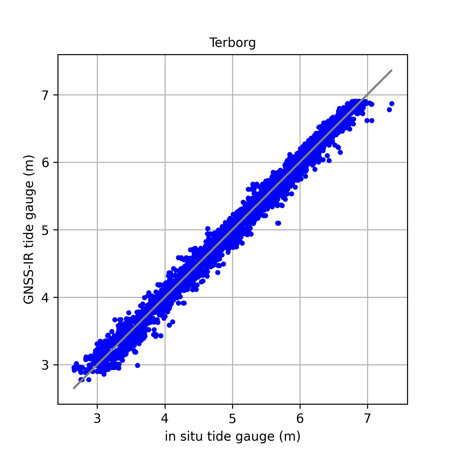
Although tracking at Terborg is limited to only three constellations, it has much better visibility of the water. This results in Terborg having nearly twice as many useable reflector heights as compared to Mornington (Fig. 10). Of the three constellations, GLONASS contributes the fewest reflector heights. This is because GLONASS has fewer frequencies than GPS or Galileo. Terborg has larger tidal variations than Mornington (nearly four meters peak to peak) and features the closure of a barrage on June 5, 2023 (Fig. 11). The agreement between GNSS-IR and the in situ tide gauge is still quite good; GNSS-IR is able to measure both tidal variations and the barrage closure. The correlation between the GNSS-IR and the tide gauge is high, 0.994, but the standard deviation of the residuals is much higher than observed at Mornington, 0.114 meters (Fig. 12).

4.4 Discussion

The difference in precision at the two sites is likely due to a combination of factors, one of which is simply that different receivers and antennas were used. It is difficult to evaluate the SNR data in more detail as few receiver manufacturers provide details about how they compute it. Although the Terborg site has a good view of the Ems river, the platform that hosts it obstructs some of the reflections; there is also more ship traffic at Terborg. Other differences are related to the GNSS- IR software. The model currently used to remove the Ḣ effect assumes relatively smooth water level changes that is clearly not ideal for the very dynamic water motions at Terborg. Eleven cm is a fairly typical precision value using the periodogram GNSS-IR method (Nievinski et al., 2020). Better precision (2–3 cm) has been reported for GNSS-IR methods that estimate hourly water levels from simultaneous rising and setting SNR arcs (Strandberg et al., 2016). However, this method also requires the water levels to have very smooth timevarying behavior which is not the case for the tidal behavior at Terborg.

gnssrefl was written to be used for retrospective data analysis, i.e. after a full day’s observations have been downloaded and translated into the RINEX or NMEA format. However, gnssrefl fully supports access to realtime multi-GNSS orbits (GFZ-orbits, 2023), meaning that in principle it would be straightforward using the existing software to update the water level time series at ~15 minute intervals. For a truly realtime GNSS-IR water level monitoring system a user would need to install an appropriate Kalman filter (Strandberg et al., 2019; Liu et al., 2023).

Here we only showed water level comparisons of three weeks. For those interested in the longterm stability of GNSS-IR, Larson et al. (2017) compared ten years of GNSS-IR water level retrievals with a NOAA tide gauge at Friday Harbor, Washington; only GPS L1 data were used. The reported standard deviation for a single GNSS-IR reflector height measurement was 12 cm, similar to what was shown for Terborg. The agreement between GNSS-IR and NOAA improved to 2 cm for daily averages and 1.3 cm for monthly averages. The tidal coefficients estimated using GNSS-IR were also in good agreement with those derived from the NOAA tide gauge. Since that study was conducted, the GPS receiver at Friday Harbor has been replaced with a multi-GNSS system that tracks modern GPS signals and multiple constellations. The new system has six times more sea level retrievals per day than the older system. Access to multi-GNSS signals is key for robust water level determination, especially if real-time measurements are desired for storm surge monitoring (Peng et al., 2019) or tsunami detection (Larson et al., 2021).

gnssrefl does not currently report water levels in ITRF. As a first step, gnssrefl does remove inter-frequency biases and reports all reflector height measurements at the L1 GPS phase center. Before adding a module in gnssrefl to define reflector heights in ITRF, comparisons at a large number of collocated tide gauge sites must be conducted. Such a study would need to ensure that accurate tie information is available for the tide gauges used as truth and should include a variety of GNSS antennas. This work is also needed to ensure that the tabular mean antenna phase centers used by the geodetic and surveying communities accurately represent the phase center for the low elevation angle data used in GNSS-IR. This activity is part of a larger International Assocation of Geodesy study group dedicated to assessing the precision and accuracy of GNSS-IR (Nievinski et al., 2020).

Although not shown here, it is important to note that significant progress has also been made in the last decade to use GNSS-IR with cheaper sensors (Strandberg et al. 2019; Williams et al., 2020; Purnell et al. 2021; Fagundes et al., 2021; Karegar et al., 2023). In addition to the obvious advantage of its lower cost, the antennas in these instances can also be modified to enhance reflections. Another potential use of GNSS-IR is on ships. There is no fundamental reason the GNSS-IR method cannot be used at sea, but it would require gnssrefl be modified to calculate azimuth and elevation angles for a moving platform. Currently gnssrefl assumes the receiver coordinates from the GNSS data files do not change.

5 Conclusions

A brief overview has been given of how the GNSS-IR technique works and how it can be used to measure water levels. For sites that have a clear and unobstructed view of the water surface and where the analyst has appropriately masked the data to remove obstructions, comparisons typically show correlations of 0.99 with traditional tide gauge sensors (Nievinski et al., 2020). Thus far the community has focused on demonstrating that GNSS-IR is capable of accurately measuring relative water levels in the short and longterm. Additional work is needed to characterize its accuracy in defining water levels in ITRF (Altamimi et al., 2023).

In regions where the primary goal of the GNSS unit is to only measure ground motion, as was the case for both our examples, a properly placed GNSS unit can provide backup water level measurements when the primary tide gauge unit fails or needs to be calibrated. A backup tide gauge can be particularly useful as traditional tide gauges can fail or be destroyed during extreme events such as storm surges and floods. GNSS-IR units need to be somewhat close to the water, but not as close as traditional tide gauges. For example, the GNSS instrument used for detecting the Shumagin earthquake tsunami is ~200 meters from the coast and ~70 meters above sea level (Larson et al., 2021).

GNSS-IR can also be used by researchers who want to use tide gauge data for geophysical and coastal studies but cannot currently do so because local ground motions (glacial isostatic adjustment, subsidence, postseismic motions) are too large (Peng et al., 2021). Researchers interested in GNSS- IR are encouraged to examine the large database of results created by the Permanent Service for Mean Sea Level (PSMSL, 2023). Despite the fact that only a handful of these GNSS sites were installed with a goal of measuring water levels, ~285 of them can be used to reliably do so. Where available, traditional tide gauge data are also shown at the web portal.

Acknowledgements

The gnssrefl software used in this study is freely available at https://github.com/kristinemlarson/gnssrefl. Documentation for the gnssrefl software is available at https://gnssrefl.readthedocs.io/en/latest/.

Mornington Island tide gauge data are provided by the State of Queensland, Department of Environment and Science¹. The RINEX files for Mornington Island were downloaded from Geoscience Australia GNSS Data Centre² using the gnssrefl software. The Terborg GNSS data are provided courtesy of Bundesanstalt für Gewässerkunde and downloaded using the gnssrefl software. The Terborg tide gauge data are provided by Wasserstraßen und Schifffahrtsverwaltung des Bundes³. Multi-GNSS orbits were provided by the Deutsches GeoForschungsZentrum⁴.

We thank T. Nischan and Y. Hatanaka for writing community software for GNSS users.

References

Altamimi, Z., Rebischung, P., Collilieux, X., Metivier, L. and Chanard, K. (2023). ITRF2020: an augmented reference frame refining modeling of nonlinear station motions, J. Geodesy, 97(47). doi:10.1007/s00190-023-01738-w

Anderson K. D. (2000). Determination of Water Level and Tides Using Interferometric Observations of GPS Signals. J Atmos Oceanic Technol., 17(8):1118–1127.

Axelrad, P., Larson, K. M. and Jones, B. (2005). Use of the Correct Satellite Repeat Period to Characterize and Reduce Site-Specific Multipath Errors, In Proc. Institute of Navigation Technical Meeting of the Satel-lite Division, Long Beach, September 2005, 2638–2648.

Bilich, A., Larson, K. M. and Axelrad, P. (2008). Modeling GPS phase pultipath with SNR: Case study from the Salar de Uyuni, Bolivia. J. Geophys. Res., 113, B04401. doi:10.1029/2007JB005194

Docker (2023). Develop faster. Run anywhere. Docker Inc. https://www.docker.com (accessed 9 Aug. 2023).

Dunne S., Soulat F., Caparrini M., Germain O., Farrés E., Barroso X. and Ruffini, G. (2005). Oceanpal: a GPS-reflection coastal instrument to monitor tide and seastate. Proceedings of the International Geoscience and Remote Sensing Symposium (IG- ARSS). Barcelona, Spain, July 23–28.

Fagundes, M., Mendonca-Tinti, I., Lescheck, A. L., Akos, D. M. and Nievsinki, F. G. (2021). An opensource lowcost sensor for SNR-based GNSS reflectometry: design and longterm validation towards sealevel altimetry, GPS Solutions, 25(73). doi:10.1007/s10291-021-01087-1

Georgiadou, Y. and Kleusberg, A. (1988). On carrier signal multipath in relative GPS positioning. Manuscripta Geodetica, 13,172–179.

GFZ-orbits (2023). Analysis center of the Multi-GNSS Experiment. https://www.gfz-potsdam.de/en/section/space-geodetic-techniques/projects/mgex/ (accessed 26 July 2023).

gnssrefl (2023). A GNSS reflectometry package. https://github.com/kristinemlarson/gnssrefl (accessed 16 June 2023).

gnssrefl-pypi (2023). A GNSS reflectometry package. https://pypi.org/project/gnssrefl (accessed 16 June 2023).

gnssir-api (2023). A GNSS-IR API. https://gnss-reflections.org/api (accessed 26 June 2023).

Karegar, M., Kusche, J., Geremia-Nievinski, F. G., Larson and K. M. (2022). Raspberry Pi Reflector (RPR): A low-cost water-level monitoring system based on GNSS interferometric reflectometry. Water Resources Research, 58(12). 10.1029/2021WR031713.

Larson, K. M., Small, E. E., Gutmann, E. D., Bilich, A. L., Braun, J. J. and Zavorotny, V. U. (2008). Use of GPS receivers as a soil moisture network for water cycle studies. Geophys. Res. Lett., 35, L24405. doi:10.1029/2008GL036013

Larson, K. M., Gutmann, E. D., Zavorotny, V. U., Braun, J. J., Williams, M. W. and Nievinski, F. G. (2009). Can we measure snow depth with GPS receivers? Geophys. Res. Lett., 36, L17502. doi:10.1029/2009GL039430

Larson, K. M., Löfgren, J. S. and Haas, R. (2013a). Coastal sea level measurements using a single geodetic receiver. Advances in Space Research, 51(8). 1301–1310, doi:10.1016/j. asr.2012.04.017

Larson, K. M., Ray, R. D., Nievinski, F. G. and Freymueller, J. T. (2013b). The Accidental Tide Gauge: A GPS Reflection Case Study from Kachemak Bay, Alaska. IEEE Geoscience and Remote Sensing Letters, 10(5), 1200–1204. doi:10.1109/ LGRS.2012.2236075

Larson, K. M. and Nievinski, F. G. (2013). GPS snow sensing: results from the EarthScope Plate Bound-ary Observatory. GPS Solutions, 17(1), 41–52. doi:10.1007/s10291-012-0259-7

Larson, K. M., Ray, R. D. and Williams, S. P. D. (2017). A 10-Year Comparison of Water Levels Meas-ured with a Geodetic GPS Receiver versus a Conventional Tide Gauge. J. Atmos. Oceanic Technol., 34(2), 295–307. doi:10.1175/JTECH-D-16-0101.1.

Larson, K. M., Lay, T., Yamazaki, Y., Cheung, K. F., Ye, L., Williams, S. D. P. and Davis, J. L. (2021). Dynamic sea level variation from GNSS: 2020 Shumagin earthquake tsunami resonance and Hurricane Laura. Geophys. Res. Lett., 48(4). doi:10.1029/2020GL091378

Liu, Z., Du, L., Zhou, P., Wang, X., Zhang, Z. and Liu, Z. (2023). Cloud-based near real-time sea level monitoring using GNSS reflectometry. GPS Solutions, 27(2), 65. doi: 10.1007/s10291-022-01382-5

Löfgren, J. and Haas, R. (2014). Sea level measurements using multi-frequency GPS and GLONASS ob-servations. EURASIP J. Adv. In Signal Processing, 50. doi:10.1186/1687-6180-2014-50

Löfgren, J., Haas, R. and Scherneck, H.-G. (2014). Sea level time series and ocean tide analysis from multipath signals at five GPS sites in different parts of the world. J. Geodynamics, 80, 66–80. doi:10.1016/j.jog.2014.02.012

Nievinski, F. G., Hobiger, T., Haas, R., Liu, W., Strandberg, J., Tabibi, S., Vey, S., Wickert, J. and Willi-ams, S. D. P. (2020). SNR-based GNSS reflectometry for coastal sea-level altimetry: results from the first IAG inter-comparison campaign. J. Geodesy, 94(70). doi:10.1007/s00190-020-01387-3

Ozeki, M., Heki, K. (2012) GPS snow depth sensor with geometry-free linear combinations. J. Geodesy, 86(3), 209–219. doi:10.1007/s00190-011-0511-x

Peng, D., Hill, E. M., Li, L., Switzer, A. D. and Larson, K. M. (2019).Applications of GNSS interfero-metric reflectometry for detecting storm surges. GPS Solutions, 23(47). doi:10.1007/s10291-019-0838-y

Peng, D., Feng, L., Larson, K. M. and Hill, E. (2021). Measuring Coastal Absolute Sea Level Changes using GNSS Interferometric Reflectoometry. Remote Sens., 13(21), 4319. doi:10.3390/ rs13214319

Purnell, D. J., Gomez, N., Minarik, W., Porter, D. and Langston, G. (2021). Precise water level measure-ments using low-cost GNSS antenna arrays. Earth Surface Dynamics, 9(3), 673–685. doi:10.5194/esurf-9-673-2021

Rost, C. and Wanninger, L. (2009). Carrier phase multipath mitigation based on GNSS signal quality measurements. Journal of Applied Geodesy, 3(2). doi:10.1515/JAG.2009.009

PSMSL (2023). GNSS-IR Site Map. Permanent Service for Mean Sea Level. https://psmsl.org/data/gnssir/map.php (accessed 12 July 2023).

Ruf, C., Chew, C., Lang, T., Morris, M. G., Nave, K., Ridley, A. and Balasubramaniam, R. (2018). A New Paradigm in Earth Environmental Monitoring with the CYGNSS Small Satellite Constellation. Scientific Reports, 8, 8782. doi:10.1038/s41598-018-27127-4

Strandberg J., Hobiger T. and Haas R. (2016). Improving GNSS-R sea level determination through inverse modeling of SNR data. Radio Science, 51(8), 1286–1296.

Strandberg, J., Hobiger, T. and Haas, R. (2019). Real-time sea-level monitoring using Kalman filtering of GNSS-R data. GPS Solutions, 23, 61. doi:10.1007/s10291-019-0851-1

Vanderplas, J. (2018). Understanding the Lomb-Scargle Periodogram. Astrophys. J. Suppl., 236(1). doi:10.3847/1538-4365/ aab766

Williams S. D. P., Bell, P. S., McCann, D. L., Cooke, R. and Sams, C. (2020). Demonstrating the Potential of Low-Cost GPS Units for the Remote Measurement of Tides and Water Levels Using Interferometric Reflectometry. J. Atmos. Oceanic Technol., 37(10). 1925-1935, doi:10.1175/JTECH-D-20-0063.1

Authors’ biographies

Kristine M. Larson received a B.A. degree in engineering sciences from Harvard University in 1985 and a Ph.D. in geophysics from Scripps Institution of Oceanography, University of California at San Diego in 1990. She was a professor of aerospace engineering sciences at the University of Colorado from 1990–2018; she is currently a professor emerita at Bonn University. She is a geodesist. She led the development of GNSS Interferometric Reflectometry. She is a Fellow of the American Geophysical Union and a member of the U.S. National Academy of Sciences.t

Simon D. P. Williams received the B.Sc. degree in geology and geophysics and the Ph.D. degree in geophysics from the University of Durham, Durham, U.K., in 1991 and 1995, respectively. From 1996 to 1999, he was a Research Assistant with the Scripps Institution of Oceanography. Since 1999, he has been a Senior Researcher with the Sea Level and Ocean Climate Group, National Oceanography Centre, Liverpool, U.K. His research interests include ground-based global navigation satellite system (GNSS) interferometric reflectometry, sea-level studies using tide gauges, GNSS and satellite altimetry, and stochastic modeling and uncertainty analysis of geophysical time series.

1. https://www.qld.gov.au/environment/coasts-waterways/beach/storm/storm-sites/mornington-island (accessed 25 Sep. 2023).
2. https://data.gnss.ga.gov.au/docs/home/index.html (accessed 25 Sep. 2023).
3. https://www.pegelonline.wsv.de/gast/stammdaten?pegelnr=3910020 (accessed 25 Sep. 2023).
4. https://www.gfz-potsdam.de/en/section/space-geodetic-techniques/projects/mgex/ (accessed 25 Sep. 2023).