1 Introduction

Hydrography is defined as the science that describes the characteristics of water bodies. Thus, according to IHO (2005), the hydrographic survey consists of carrying out various measurements, such as tides and depth values. The main objective of a hydrographic survey is to compile data for building or updating nautical charts and publications.

The Brazilian Navy is responsible for producing, editing, and publishing Brazilian nautical charts and carrying out hydrographic surveys in Brazilian Waters. However, private companies are registered and authorized to collect and process bathymetric data for cartographic purposes. In this context, these companies must follow the guidelines stipulated in the NORMAM-25 (DHN, 2017) and S-44 (IHO, 2008).

Hydrographic surveys intended, for example, towards nautical cartography or port works, must fully comply with the specifications provided by Special Publication S-44, 5th edition (IHO, 2008; DHN, 2017). In this sense, the S-44 specifies four orders: Special Order, Order 1a, Order 1b, and Order 2. The International Hydrographic Organization (IHO) has already developed the sixth edition of S-44, which contains a fifth survey order, more restrictive than the special order, called the exclusive order (IHO 2020), summarized in Table 1.

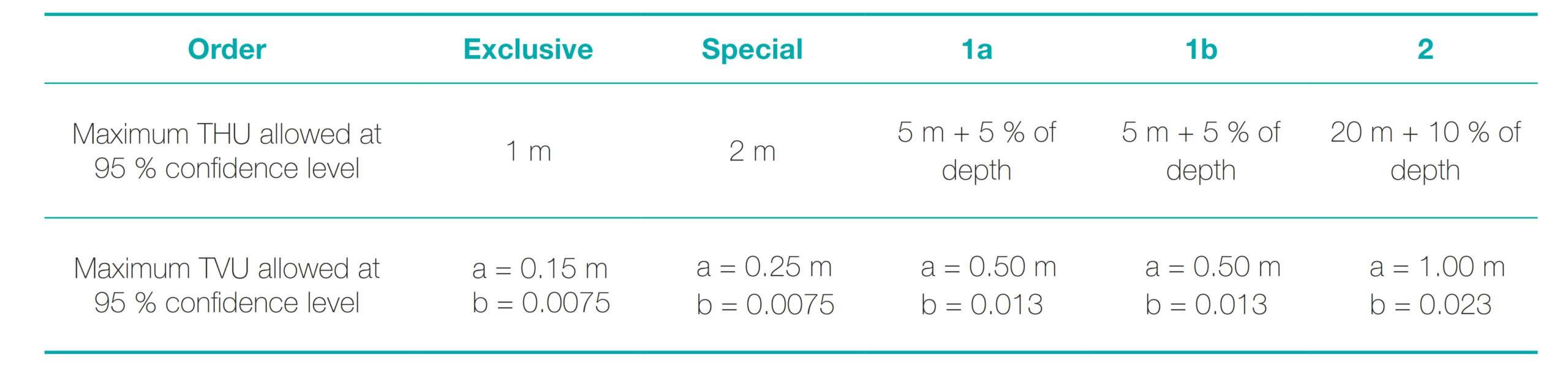
In Table 1, Order 2 represents some areas where a general description of the seafloor is considered adequate. Order 1b considers areas under keel clearance not an issue for the type of surface shipping expected to transit the area. The 1a is for places where under-keel clearance is critical. Still, features of concern to surface shipping may exist. Therefore, the special order represents areas under keel clearance is critical, and the last, Exclusive Order, considers areas with a strict minimum under keel clearance and maneuverability criteria.

The parameter a means the uncertainty portion that does not vary according to the depth, and b is a coefficient representing that uncertainty portion that varies according to depth.

The THU and TVU parameters correspond to the total horizontal and vertical uncertainties of the bathymetric data and can be obtained in two ways. The first consists of assessing all sources of uncertainty in the survey system and, subsequently, applying the uncertainty propagation law (covariance) as performed by Hare (1995) and Ferreira et al. (2016a). Although the methodology is widely used, it can only estimate the survey quality by analyzing the possible theoretical uncertainties of the components (hardware) of the sounding system (IHO, 2005; LINZ, 2010; Ferreira et al., 2016a). These uncertainties are classified as a priori (Ferreira et al., 2016b). The second one, considered the most appropriate, estimates the sampling uncertainty (a posteriori) based on “redundant” information in the same way that is carried out in surveying geodetic, topographic, and aero-photogrammetric data. Since obtaining redundancies or similar points in hydrographic surveys are generally unavailable, theoretical and practical equipment is used for these estimates. In the TVU case, which is the focus of this study, check lines (CL) crossing the sounding lines (SL) were used. Thus making it possible to obtain homologous points (the same depth value for the point on the CL and the point on the SL) and, subsequently, to calculate discrepancies and sample uncertainty.

Check lines are used for the vertical quality evaluation of depths collected by single-beam echosounders. However, due to the massive amount of data produced during the survey with multibeam sonars, the methodology used to obtain the discrepancy samples presents specific difficulties and, therefore, requires a different approach. The most common way to generate these samples is to produce digital depth models from the data, composed of sounding and check lines. The digital models from each track are compared pixel by pixel to generate a discrepancy file (Susan & Wells, 2000; Souza & Krueger, 2009; Eeg, 2010). However, digital models result from mathematical and/or geostatistical interpolations, presenting uncertainties in their estimates (Ferreira et al., 2013, 2015), compromising the quality of hydrographic survey analysis.

Souza & Krueger (2009) used data from a multibeam system to generate a bathymetric model and respective sample uncertainty. This system was able to create a vertical uncertainty expectation of ±0.240 m. However, the smallest interval of sampling uncertainty in the hydrographic survey, with a 95 % confidence level, had its variation around ± 0.305 m, which demonstrates the existence of uncertainties that were not quantified and that possibly came from the interpolation process. Nascimento (2019) concluded that, by interpolating data in cells with dimensions above the planned spacing, it is possible to establish a safety margin for the interpolation of a surface without the occurrence of empty cells, using LiDAR data, with a spacing of 3 m × 3 m and double sweep (200 % coverage).

It should be noted that check lines do not indicate absolute accuracy since data are collected normally from the same survey platform. In this case, there are sources of potential and common uncertainties between the data obtained by the sounding and check lines. However, when a submerged strip is swatted again, either by verification or adjacent swaths, it is expected that the reduced depths are distributed around the real (unknown) depth. That is, information can be a good potential survey vertical quality indicator as long as the collected data receives coherent statistical treatment.

In this sense, this study applies three methods (Surface-to-Surface, Surface-to-Point, and Point-to-Point) to compare the depth found using the SL and CL. The work aims to validate the P2P method as a valuable tool to be used in MBES data without the need to use interpolators in the data. It also presents itself as an open tool with free access.

2 Materials and method

Specific methods are required to obtain discrepancy samples in the multibeam survey process (for example, beamformers or interferometers). Within this context, the present study addresses the application of three methods, here called Method SS (Surface-to-Surface), Method SP (Surface-to-Point), and Method P2P (Point-to-Point).

The flowchart in Fig. 1 summarizes the techniques used to obtain the discrepancy samples using the three methods covered in this study.

The SS method consists of the bathymetric model creating regular probing and verification swaths. The depths are compared pixel by pixel, aiming at the discrepancy file production (Souza & Krueger, 2009). This method depends on the bathymetric model resolution; that is, the number of discrepancies and the quality of the analysis are directly linked to the pixel size used in the interpolation process (Ferreira, 2018). Another method applied is the Surface-to-point, or SP method, which uses only a bathymetric surface obtained through an interpolation process and generated from regular probing swaths, reducing uncertainties associated with the interpolation process. After generating the surface, it is compared with the depths calculated from the check lines to obtain the discrepancies. In the SP method, the sample size of the discrepancy file is proportional, above all, to the density of the point cloud of the verification swaths. The quality of the analysis depends on the data collected and their respective resolutions.

In another approach, in the P2P method, the discrepancy file is obtained by comparing sounding lines and check lines without using interpolation methods (Ferreira, 2018).

The P2P method is the main study object of this work. The first step is the application of filtering or cleaning the depth of the data collected. Then, the SL and CL are used as data input to the algorithm. After reading the SL, the intersection area between them is identified. Then, after extracting the respective points present in swaths, the algorithm uses a limited distance to search for the nearest neighbor and to find a probable homologous point on the SL with this limited distance.

So, after identifying the homologous points between the CL and SL, the P2P method calculates the discrepancies of the homologous points. With the generation of the discrepancy files, it is possible to analyze the vertical quality of the hydrographic survey.

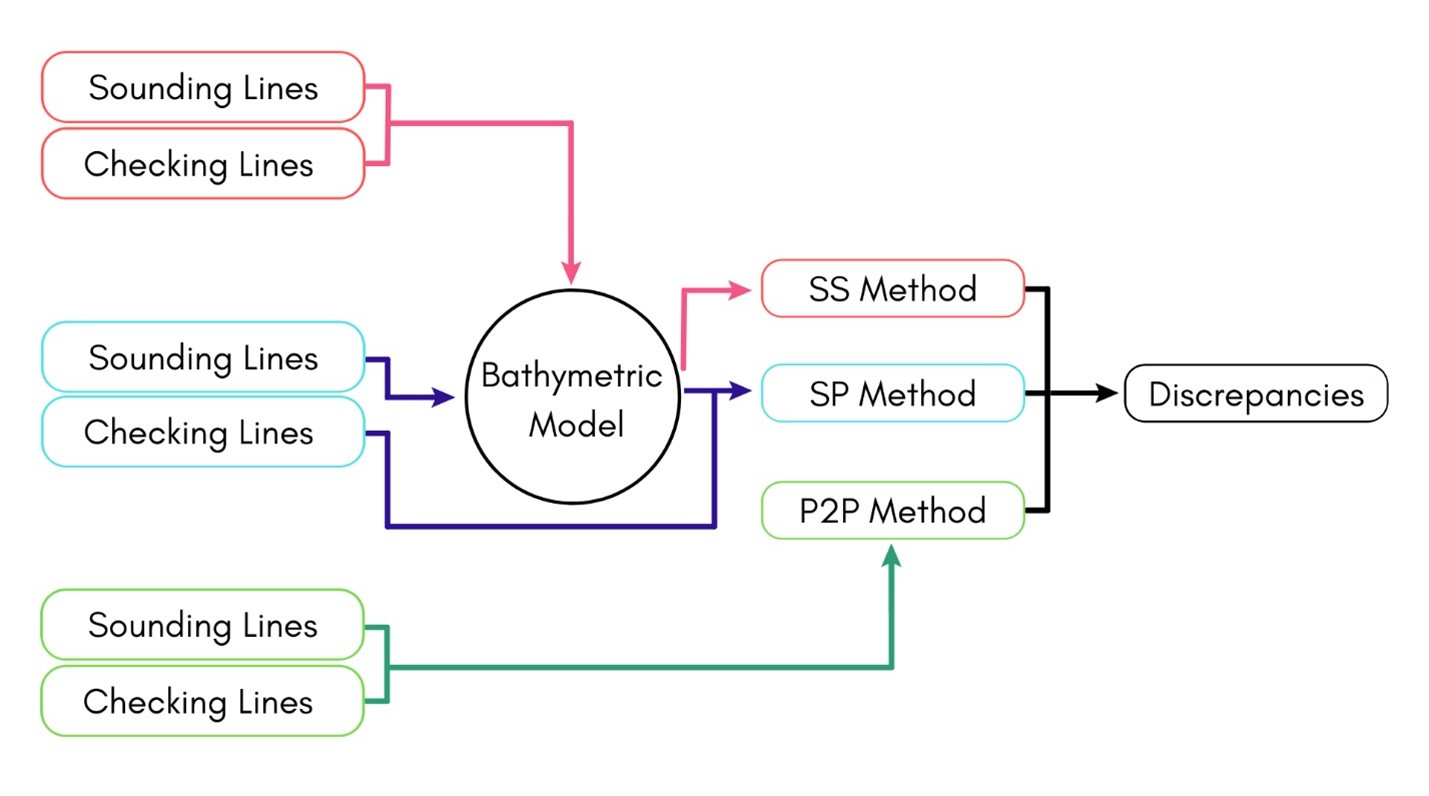
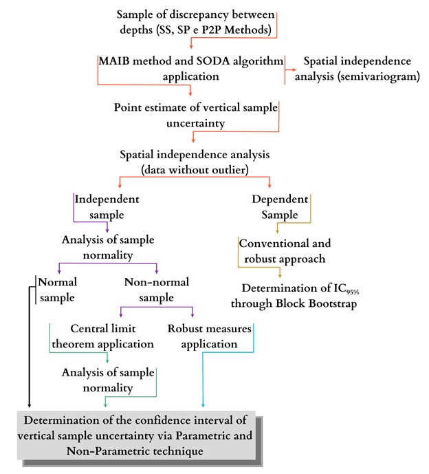
Fig. 2 illustrates the methodology flowchart used to assess the vertical data quality through the discrepancies obtained by the three methods covered in this study. It should be noted that the applied methodology is based on basic theorems of classical and geostatistical methods, both implemented in software R (R Core Team, 2017).

Firstly, the georeferenced discrepancy samples were imported by the algorithm. The file must have positional coordinates X, Y (whether local, projected, or geodetic), depth (Z), and the discrepancy between “homologous depths” (dz).

The next step was to carry out the exploratory analysis of the discrepancy samples, which sought the presence of outliers within the data distribution with the aid of the SODA (Spatial Outliers Detection Algorithm) algorithm (Morettin & Bussab, 2004; Ferreira et al., 2013; Ferreira et al., 2019a; Ferreira et al., 2019b). This algorithm performs the detection of spikes and outliers in the bathymetric data collected by swath-sounding systems using different identification techniques or thresholds, namely the Adjusted Boxplot (Vandervieren & Hubert, 2004), Modified Z-Score (Iglewicz & Hoaglin,1993), and the δ method. The latter was partly inspired by Lu et al. (2010), which applies spike detection thresholds based on the variances of subsamples.

At this stage, MAIB (Methodology for the Assessment of Uncertainty of Bathymetric data), proposed by Ferreira (2018), basically interprets the graphs produced (histograms, boxplot, Q-Q Plot, etc.), as well as does statistical analysis (mean, variance, minimum, maximum, asymmetry coefficients, and kurtosis, etc.). In general, the MAIB algorithm was developed to assess the vertical quality of bathymetric surveys through observations collected in the check lines, addressing issues about the independence and normality of the data and the presence or absence of outliers.

The next phase of the MAIB application estimated the vertical uncertainties by applying specific measures of theoretical accuracy through the analysis of RMSE (Root Mean Square Error) and ϕ_Robust (Mikhail & Ackerman, 1976; Ferreira et al., 2019a). The last method was created by Ferreira et al. (2019a) and uses the median (Q2) and the NMAD (Normalized Median Absolute Deviation) to estimate vertical uncertainty. ϕ_Robust consists of the square root of the sum of the square of Q2 and the square of NMAD.

Constructing statistically optimal confidence intervals is necessary to evaluate the data distribution and spatial autocorrelation. In this context, the next step was to analyze sample independence. For this, we opted to use the semi-variogram, a robust tool used by geostatistical to evaluate the spatial data autocorrelation (Matheron, 1965).

After the independence between the discrepancy samples was verified, normality tests were used. In this work, the Kolmogorov-Smirnov (KS) test was used at the 95 % confidence level since the Shapiro-Wilk application is limited to samples with up to 5,000 points (Filho, 2013). The KS test assesses the similarity between sample and reference distributions. The main purpose is to determine whether evidence suggests that the two distributions significantly differ from each other (Doob, 1949). If the test provides a p-value > 0.05 as a response, the sample is said to be normal at the 5 % significance level. Therefore, from this stage onwards, MAIB suggests subdividing the analysis into three categories: independent and normal samples, independent and non-normal samples, and dependent samples. The final step consisted of processing the data obtained for each category subdivided by MAIB.

In the case of samples that showed to be dependent, the 95 % confidence interval was determined using Block Bootstrap, as described in (Lahiri, 1999; Lahiri, 2003; Lee & Lai, 2009; Kreiss & Paparoditis, 2011). The Block Bootstrap method is a sampling approach to estimate the significance of the statistics test (Efron & Tibshirani, 1993; Davison & Hinkley, 1997; Zoubir, 2004; Mudelsee, 2010). This study used an R environment to implement the methodology and the rest. In the algorithm, the user must provide the block’s diagonal size and the number of bootstrap replications. The diagonal is proposed to be equivalent to the distance within which the data are correlated, the range. Furthermore, replications must exceed 500 (Ferreira, 2018).

3 Results

From the hydrographic survey carried out in the region of Porto in Rio de Janeiro, between Enxadas Island and Cobras Island (Fig. 3), it was possible to obtain the bathymetric data that served as a basis for applying the above-proposed methodologies.

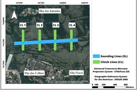
The raw data were collected using a swath system composed of a multibeam echosounder (R2 Sonic 2022) with a frequency of approximately 200 kHz. Three adjacent regular swaths were used (summarized in an SL file), and four CL. SL and CL were first pre-processed in the Hysweep software (Hypack, 2020). Then, the three-dimensional coordinates in XYZ format were obtained after analyzing and correcting latency, sound speed, attitude, and tide.

The study area has a flat submerged bottom, with few variations, and it should be mentioned that the SL and CL sounded in the same survey.

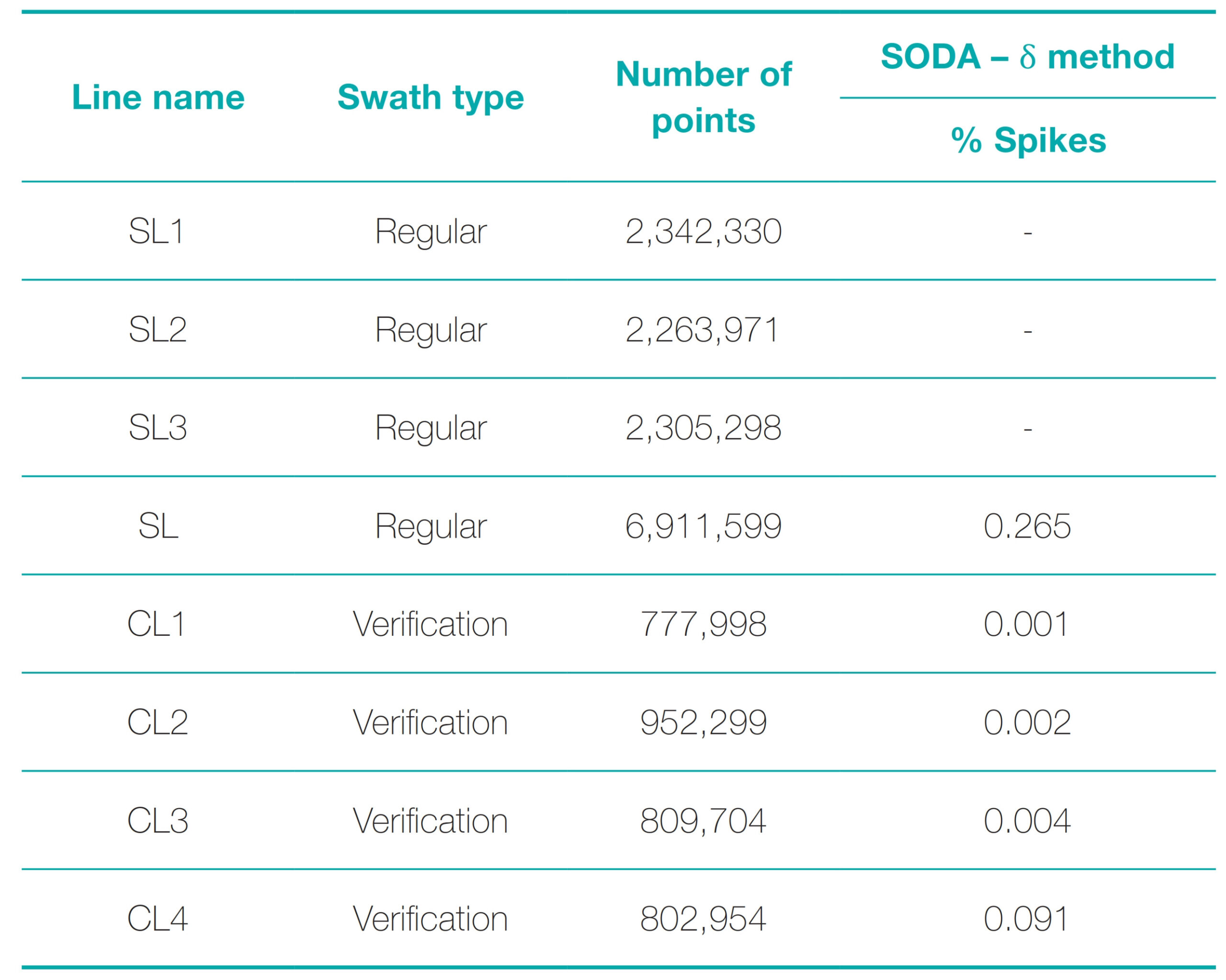
The sounding lines were gathered into a single SL file (Table 2). The files were used to obtain the results to be analyzed later.

The last column shows the percentage of spikes found and are configured as spurious depths (outliers) in hydrographic surveys. The SODA algorithm was briefly used to detect spikes in this phase, which uses the δ method to identify spurious depths (Ferreira, 2018; Ferreira et al., 2019). It can be said that performing spatial modeling without trend and with minimal variance can strengthen the spike detection technique.

After obtaining the three-dimensional coordinates, the methods for acquiring discrepancy files were developed according to the steps illustrated in Fig. 2. In this context, a geostatistical analysis was first performed to generate the bathymetric models. This analysis was followed by Simple Kriging, which aimed at standardizing the data. It should be noted that the resolution of a bathymetric model must be half the size of the smallest object intended to be detected/ represented. In this study case, for hydrographic surveys of Special Order, where the detection of cubic structures with 1 cubic meter is a mandatory edge, the bathymetric surface resolution must be greater than 0.5 m (IHO, 2008; Vicente, 2011).

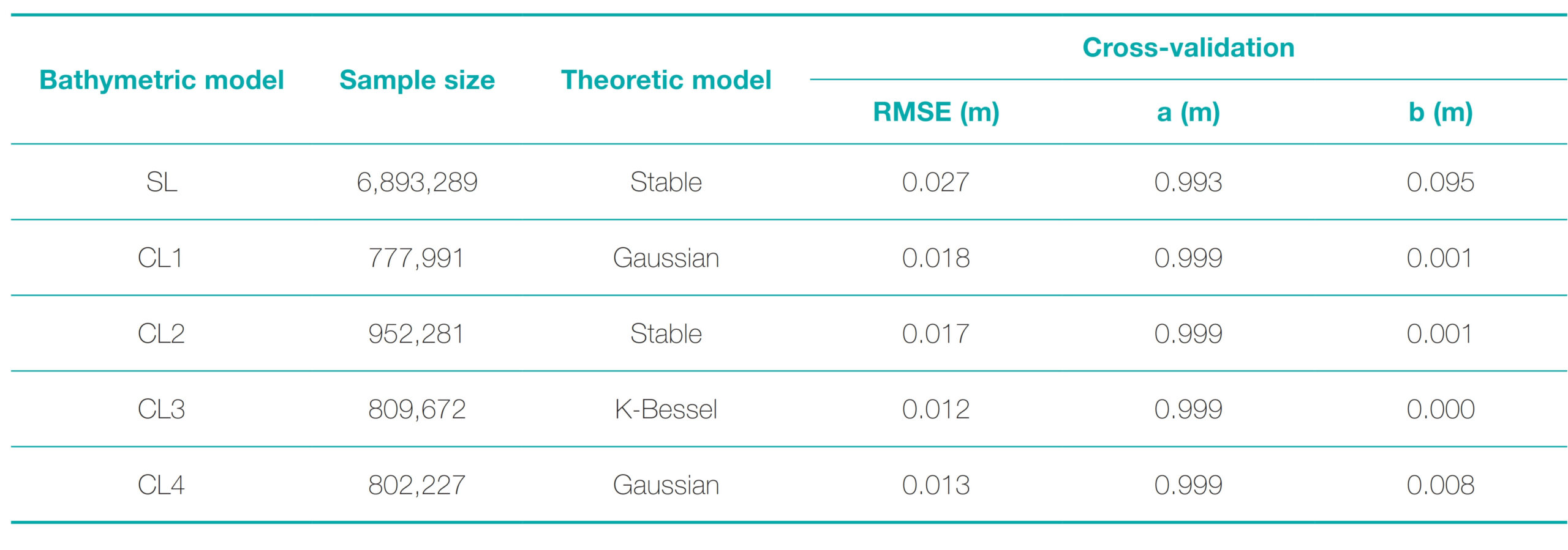
According to (Viera, 2000) and (Ferreira et al., 2013), after geostatistical modeling, it is recommended to use a cross-validation process, for example, self-validation or leave-one-out. Vieira (2000) affirms that through cross-validation, it is possible to obtain different statistical indicators (standard error, sum of the residuals’ squares, and determination coefficient R2), which assess the quality of geostatistical analyses. The results obtained are available in Table 3.

The theoretical model indicates which type of kriging adjustment better suits the sample inserted in the algorithm. Then, the methods for obtaining the discrepancy samples were applied from the bathymetric models. The discrepancy files obtained correspond to the intersection area of each of the four check lines with the sounding line (Fig. 3).

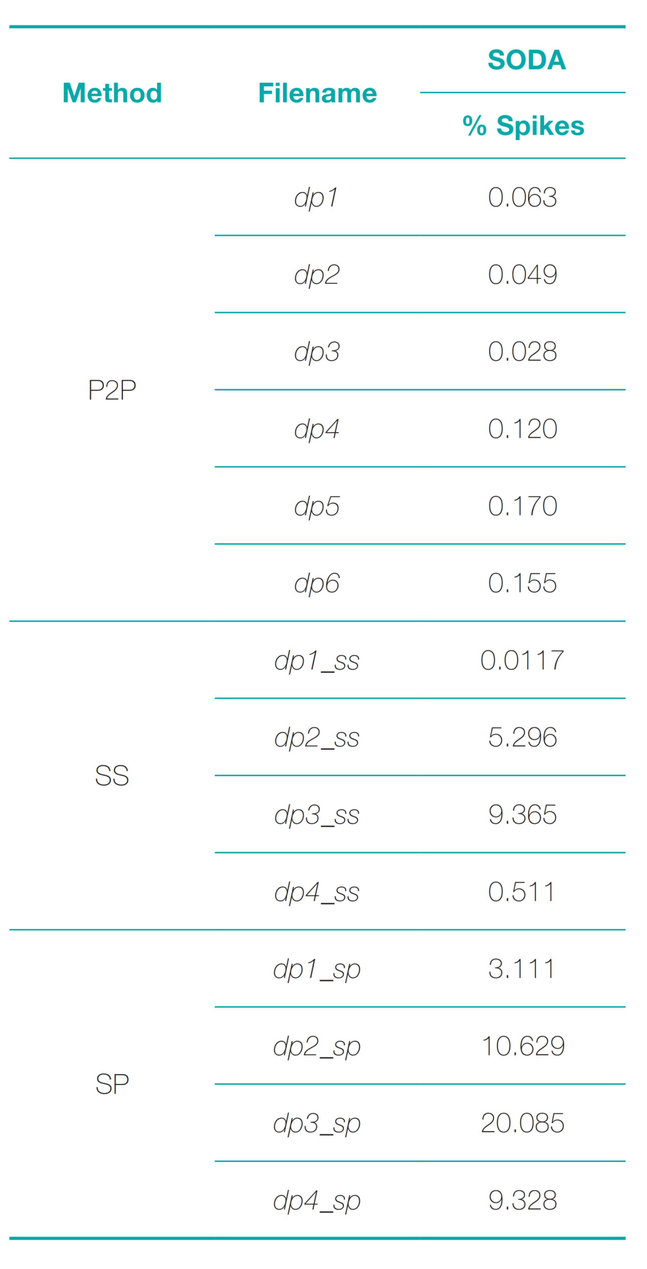
For the P2P method, in addition to the discrepancies obtained through the intersections between the SL and the CLs (dp1, dp2, dp3, and dp4), discrepancies were also obtained from the sounding lines overlap, which resulted in the dp5 and dp6 files. For the SS method, the bathymetric grids were compared and obtained the discrepancies files dp1_ss, dp2_ss, dp3_ss, and dp4_ss. Finally, in the case of the SP method, the bathymetric model constructed based on regular sweeps was compared with the depths calculated through the check lines. This comparison resulted in the discrepancies in files dp1_sp, dp2_sp, dp3_sp, and dp4_sp.

The discrepancy files were submitted to the SODA methodology developed by Ferreira et al. (2019a) for outlier detection. The methodology underwent changes when it was used to investigate the discrepancy. More information on the use of the SODA methodology can be seen in the research done by Ferreira (2018) and Ferreira et al. (2019a).

It should be noted that the geostatistical analyses were used to generate standardized residues (SRs) when the user noted a spatial autocorrelation. Thus, the search for discrepancies was applied to the SRs, as mentioned in the SODA methodology. The search radius was three times the distance in all analyses. Table 4 summarizes the results obtained at this processing stage. Notably, the δ Method is based on the median (Q2) and the constants c and δ. The constant c takes the value 1 for irregular reliefs with high variability, 2 for wavy reliefs (medium variability), and 3 for flat reliefs. The user must enter this value. The algorithm automatically determines the constant δ by evaluating the Global Normalized Median Absolute Deviation (NMAD).

After applying the SODA methodology, the MAIB analysis was performed. As this work compares the traditionally applied methods with the methodology developed by Ferreira (2018), a summary of the traditional analysis carried out based on S-44 tolerances (IHO, 2008) is shown in Table 5. In addition, this table also presents the values of RMSE and ϕ_Robust that served as a basis to compute the vertical sample uncertainty (Ferreira et al., 2019b).

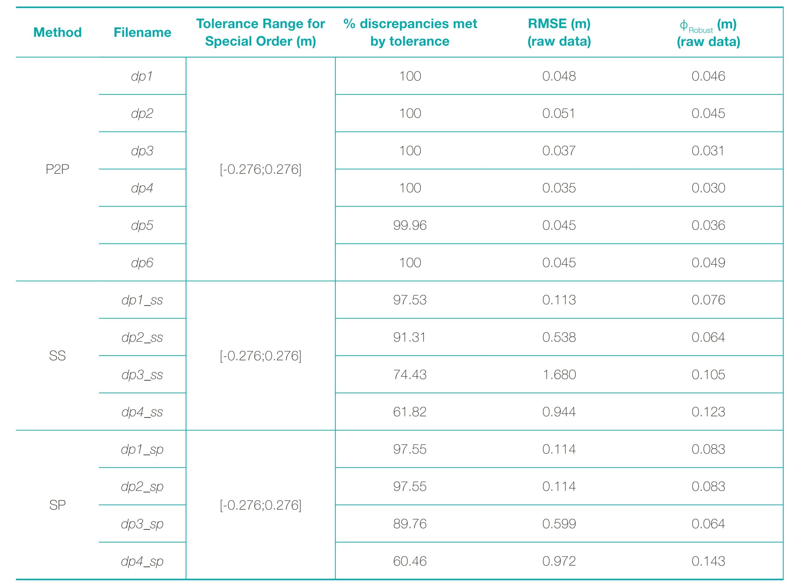
The dp5 and dp6 samples were used to evaluate and validate an estimate of the sampling uncertainty obtained by the overlap between sounding lines. The other samples (dp1, dp2, dp3, and dp4) presented, on average, 99.99 % of the discrepancies with values below the tolerance stipulated in S-44. The same average value was found for samples dp5 and dp6.

For sample uncertainty point estimation with the RMSE and ϕ_Robust, the dp5 and dp6 samples had mean values of 0.045 m and 0.043 m, respectively. The values are mathematically equivalent compared to results obtained through the check line surveys. It should be noted that the dp6 sample obtained a value of ϕ_Robust higher than the value of RMSE, something quite unusual but possible to occur. It was observed that this occurred mainly due to the nature of the frequency distribution of the data set used, explaining this change.

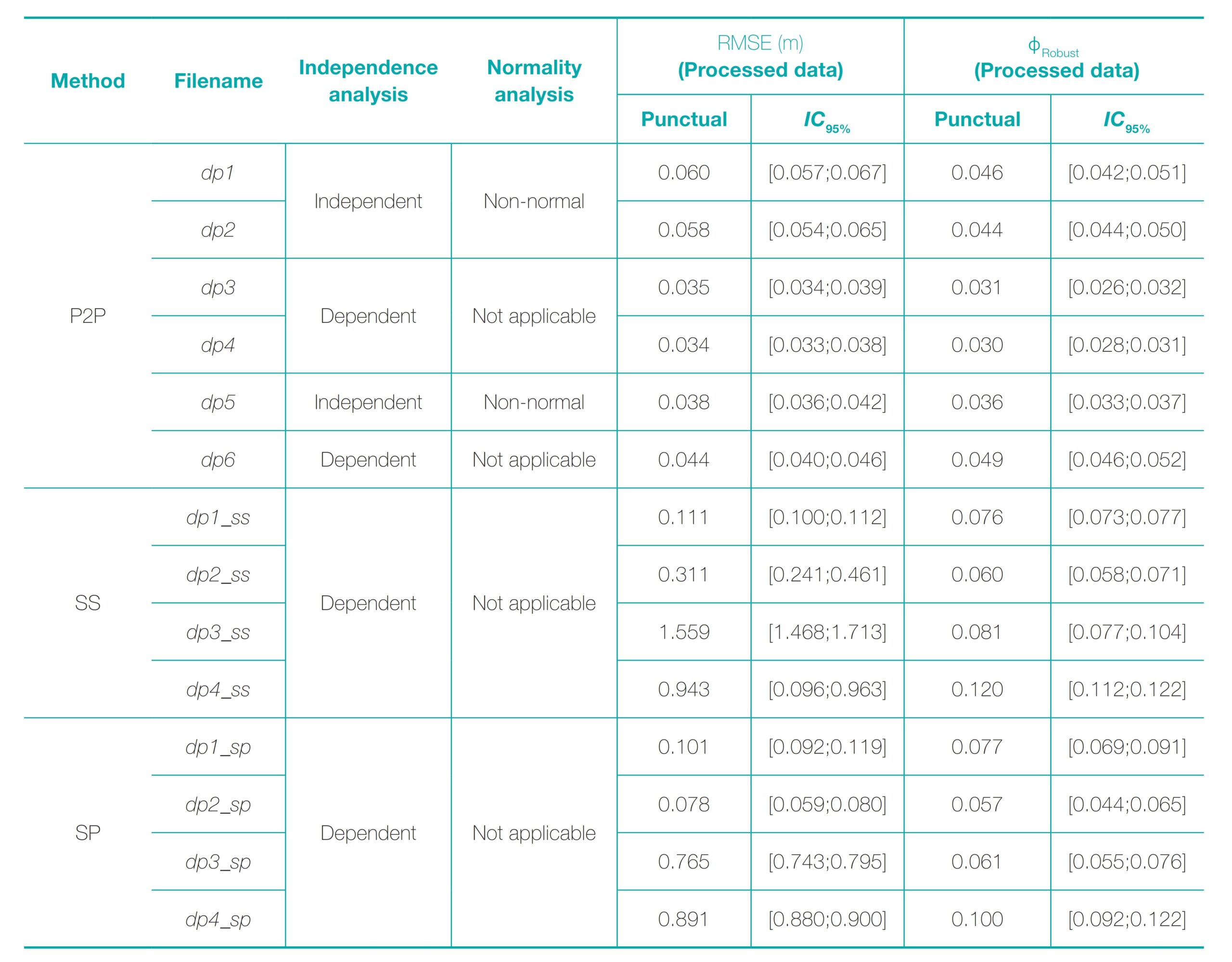
After that stage, we proceeded to the last data evaluation process with the continued application of the MAIB methodology. The results obtained are described in Table 6.

4 Discussion

4.1 Bathymetric model uncertainty and outlier detection

From the data in Table 3, the generated bathymetric models have low uncertainty. This conclusion is supported by the values of RMSE, Average Error, and coefficient b which consistently exhibit null or near-zero values. In contrast, coefficient a consistently exceeds 0.99 m across all models.

Shifting the focus to applying the SODA algorithm for outlier detection (Table 4), attention is drawn to the sample dp1_ss, demonstrating the lowest proportion of outliers. Among the 29,792 discrepancy samples obtained, only 35 (equivalent to 0.12 % of the entire set) were flagged as anomalous. Conversely, the dp3_sp sample showcases a contamination percentage surpassing 20 %. Among the diverse methods scrutinized in this study, the P2P method yields the most modest proportion of outliers. This observation aligns with the notion that the magnitude of outliers is directly correlated with the sample size of the dataset.

4.2 Comparative analysis of methods

Turning to the outcomes presented in Table 5, it becomes evident that employing the P2P method results in the classification of the survey under the Special Order category. On average, a remarkable 99.99 % of discrepancies fall within the tolerance set by S-44. However, recognizing the susceptibility of the RMSE estimator to outliers, preference is given to the ϕ_Robust estimator for its superior suitability (Ferreira et al., 2019b). This choice is reinforced by the ϕ_Robust estimator’s average sample uncertainty of approximately 0.038 m. Considering the parallel evaluation of average sample uncertainty values obtained through both estimators, it becomes apparent that these values affirm the quality of the collected data within the study area and validate the effectiveness of the P2P method.

4.3 Validation of proposed methodology

Directing attention to the SS method, an initial analysis might suggest that, prima facie, the hydrographic survey may not align with the intended order. This inference arises from the sole instance (dp1_ss) exhibiting more than 95 % of discrepancies within the S-44 stipulated tolerance range. However, upon analyzing the average of discrepancies across all four files, only 81.27 % of values fall within the S-44 range. As for the sample uncertainty point, the estimator yields an average of 0.819 m for RMSE and 0.092 for ϕ_Robust. Discrepancies between these values hint at outliers masking the accuracy of vertical bathymetry analysis. The most substantial discrepancy between estimators is evident in the dp3_ss sample, exhibiting a notable 1.575 m difference, followed by dp4_ss, dp2_ss, and dp1_ss.

Comparable results of a similar order of magnitude emerge from the SP method as in the SS method. The SP method showcases a solitary instance (dp1_sp) aligning with the tolerable range for Special Order in percentage. On average, around 80 % of discrepancies fall within the 95% confidence interval specified by S-44, suggesting a misalignment of the survey with the intended order. Notably, the point uncertainty estimates (RMSE and ϕ_Robust) average 0.906 m and 0.098 m, respectively. Analogous to the SS method, the most pronounced difference is observed in the dp3_sp sample, trailed by dp4_sp, dp2_sp, and dp1_sp samples. This prompts a parallel application of considerations similar to those applied to the SS method.

Considering the analysis encapsulated in Table 6, the divergent outcomes attributed to the methods used for obtaining discrepancy samples can be rationalized. The SP and SS methods, grounded in mathematical interpolators, deviate due to the geostatistical methods employed in this study (Ferreira, 2018). Based on the obtained outcomes, emphasis is warranted on the P2P method, which is recommended for traditional hydrographic survey analyses.

Among the samples employed within the P2P-method, spatial independence is evident in three cases (dp1, dp2, and dp5). Subsequently, the Kolmogorov-Smirnov (KS) normality test is applied at the 95 % confidence level. This test underscores the lack of adherence to normality, attributed to a p-value ≈ 0. Consequently, the Central Limit Theorem (CLT) takes precedence (Ferreira, 2018; Ferreira et al., 2019b). The CLT posits that, with a growing sample size, the sample mean distribution tends towards a standard normal distribution (Fischer, 2010). The formation of groups is realized by opting for a cluster size of 4, denoting the minimum number of elements advised for a group, and employing Euclidean distance for dissimilarity assessment (Reynolds et al., 1992). This culminates in deriving the average of discrepancies for each group to establish CLT samples from the database.

Concluding from the results spotlighted in Table 6, the P2P method emerges as a more coherent and efficacious choice than the SS and SP methods. Notably, a conspicuous pattern arises by juxtaposing the data involving outlier presence (Table 5) with the outlier-free bases (Table 6). Specifically, the mean ϕ_Robust values stand at null for the P2P method, 0.008 for the SS method, and 0.024 for the SP method. These outcomes underscore the supremacy of the proposed method, underpinned by the theoretical premise that the mean difference in ϕ_Robust statistics should be null, irrespective of the presence of discrepant data.

Regarding RMSE values, the P2P, SS, and SP methods exhibit averages of -0.007 m, 0.088 m, and 0.447 m, respectively. Susan & Wells (2000) and Eeg (2010) have previously applied the RMSE estimator to gauge survey uncertainty and classify it in line with S-44. More significant differences were expected in this analysis since outliers highly influence the RMSE estimator. A plausible rationale attributes this variation to the superior data quality collected. However, it is noteworthy that the P2P method presents the most distinct value among the analyzed methods, suggesting that estimates derived from outlier-derived data are comparatively lower than those found in the proposed methodology. The evidence corroborates the estimates produced by CLT in the case of samples dp1 and dp2.

Referring to the results presented in Table 6, even with excluding outliers, the RMSE outcomes for dp1 and dp2 samples mathematically surpass those computed via the traditional method outlined in Table 6. This discrepancy is rooted in the CLT’s behavior (Fischer, 2010). Applying this theorem tends to amplify the point estimate of sample uncertainty. Conversely, confidence interval estimates exhibit marked consistency and reliability.

Analyzing the dp3 and dp4 samples through the lens of the P2P method, one observes close alignment with outcomes derived from the traditional method. However, variance in confidence intervals persists. While RMSE values suggest convergence or near-convergence, such proximity masks the contribution of outliers. Conversely, ϕ_Robust values highlight the effect of high-quality data coupled with the P2P method’s robustness. Rooted in the proposed methodology and study development, the surveyed domain can be classified within the Special Order/ Category A, per the adopted regulations. These outcomes materialize upon the application of the traditional method. Notably, the generation of these integral intervals is uniquely attributed to the methodology advanced in this work.

In the case of the SS method, the dp2_ss and dp3_ss samples, encompassing both outlier-rich and outlier-free datasets, yield RMSE estimates that significantly diverge. However, concerning the ϕ_Robust estimator, barring the dp3_ss sample, all bases yield either millimeter or zero disparities. Leveraging the Block Bootstrap method, the confidence intervals constructed for both SS and SP methods attest to their accuracy and high quality. Occasional inconsistencies in the 95 % confidence intervals, as anticipated, prompt iterative recalibration by augmenting the number of bootstrap replications. Regarding normative classification, aligning with Special Order and Category A, the survey’s outcome remains consistent with traditional analysis. A robust approach, collectively and individually, engenders 95 % confidence interval estimates.

Comparatively, the SP method yields less promising results. Contrasting RMSE values exhibited in Tables 5 and 6, an average difference of approximately 50 cm surfaces. This disparity signifies the prevalence of outliers within this method, potentially obfuscating the evaluation of hydrographic survey vertical quality (Ferreira, 2018). When analyzed individually, all samples exhibit substantial disparities. However, the robust estimator paints a more optimistic picture for the SP method. Nevertheless, juxtaposed against the other examined methods (SS and P2P), the SP method’s inefficiency manifests. Notwithstanding, the values generated through the Block Bootstrap method retain consistency and reliability for the SP method.

Finally, upon applying the SP method for the S-44 (IHO, 2008) classification, only the ϕ_Robust estimator yields results consistent with the Special Order. Regarding RMSE, at the 95 % confidence level, outcomes reveal that samples dp1_sp and dp2_sp feature intervals align with S-44 stipulated tolerances. However, the general average across all four files deviates, implying the survey is classified in the desired order and class.

The effort to validate interval estimation is evident in evaluating sampling uncertainty via overlapping sounding lines at the 95 % confidence level. To this end, dp5 and dp6 samples were generated, where dp5 showcases sample independence. Despite applying CLT yielding unanticipated outcomes, reliance on the robust approach offers a viable estimation of sampling uncertainty and confidence intervals. However, it is pertinent to note that the conventional approach’s reliability could be more robust. Analysis of RMSE estimates (Tables 5 and 6) underscores the dp6 sample’s mere 1 mm disparity.

For the dp5 and dp6 samples, the ϕ_Robust estimator yields congruent outcomes across the analyzed sets. Evaluating bathymetric survey quality via check lines yields a robust estimator-estimated point uncertainty equivalent to 0.039 m. In contrast, the successive SLs generate a value of 0.044 m, indicating a mere 5-millimeter disparity. Notably, the confidence intervals remain statistically equivalent in amplitude across both scenarios. This substantiates the evaluation’s feasibility, accuracy, and consistency via adjacent overlap of sounding lines, rendering it a practical and implementable alternative.

5 Conclusion

The main objective of this study was to propose a new technique for homologous depth extraction collected through swath systems called the P2P method. This new technique was compared to the methods commonly used among the hydrographic community (SS and SP). Through a thorough investigation, it was possible to verify greater accuracy and consistency of the P2P method through the values obtained for RMSE and ϕ_Robust, highlighted in Tables 5 and 6, in all the analyzed cases.

After evaluating the hydrographic survey in question, known to be classified in Category A/Special Order, it was possible to verify that, using only the discrepancy data generated by the application of the P2P method, results were generated capable of classifying the survey in the intended category/order. The SP and SS methods reflected the real quality of the bathymetric data associated with the robust estimator proposed by Ferreira et al. (2019c).

Therefore, the P2P method is suggested for generating discrepancies, given that the other methods (SS and SP) proved ineffective. Thus, the results generated by applying the proposed method allowed us to conclude the superiority of the P2P method.

Another problem related to traditional methods (SS and SP) is that they produce more homologous points, which results in time-consuming computational analyses. Added to this is that the SS and SP techniques are based on bathymetric models, which adds uncertainty to the process, generating flawed analyses.

As for the vertical quality analysis with the discrepancies of the overlapping of successive sounding lines, it was concluded that such a method is effective and applicable. Thus, the realization of check lines, in general, is dispensable. Therefore, it was possible to conclude that the objective of this study was achieved since the methodology developed is appropriate, accurate, and consistent.

The study in question deals with unpublished proposals, indicating what improvements should be made. For future work, it is suggested to perform upgrades in the developed algorithm to minimize the computational processing time. Implementing the algorithm within a GIS (Geographic Information System) software is recommended, allowing the user to perform the processing semi-automatically without exporting data to a text file. In addition, further studies are also recommended on the successive overlap of regular swaths in different study areas.

References

Davison, A and Hinkley D. (1997). Bootstrap Methods and Their Application. Cambridge Univ. Press: Cambridge, New York. DHN (2017). NORMAM 25: Normas da Autoridade Marítima para Levantamentos Hidrográficos. Diretoria de Hidrografia e Navegação, Marinha do Brasil, Brasil, 52p.

Doob, J. L. (1949). Heuristic approach to the Kolmogorov-Smirnov theorems. The Annals of Mathematical Statistics, 20(3), 393–403. Eeg, J. (2010). Multibeam Crosscheck Analysis: A Case Study. The International Hydrographic Review, 4, 25–33.

Efron, B. and Tibishirani, R. J. (1993). An Introduction to the Bootstrap. New York: Chapman & Hall, 436p.

Ferreira, Í. O. (2018). Controle de qualidade em levantamentos hidrográficos. Tese (Doutorado). Programa de Pós-Graduação em Engenharia Civil, Departamento de Engenharia Civil, Universidade Federal de Viçosa, Viçosa, MinasGerais, 216p.

Ferreira, Í. O., Santos, A. P., Oliveira, J. C. Medeiros, N. G. and Emiliano, P. C. (2019a). Robust Methodology for Detection of Spikes in Multibeam Echo Sounder Data. Bulletin of Geodetic Sciences, 25(3): e2019014.

Ferreira, Í. O., Emiliano, P. C., de Paula dos Santos, A., das Graças Medeiros, N. and de Oliveira, J. C. (2019c). Proposição de um Estimador Pontual para Incerteza Vertical de Levantamentos Hidrográficos. Revista Brasileira de Cartografia, 71(1), 1–30.

Ferreira, Í. O., Neto, A. A. and Monteiro, C. S. (2016a). The Use of Non-Tripulated Vessels in Bathymetric Surveys. Revista Brasileira de Cartografia, 68(10), 1885–1903.

Ferreira, Í. O., Rodrigues, D. D, Neto, A. A. and Monteiro, C. S. (2016b). Modelo de incerteza para sondadores de feixe simples. Revista Brasileira de Cartografia, 68(5), 863–881.

Ferreira, Í. O., Rodrigues, D. D. and Santos, G. R. (2015). Coleta, processamento e análise de dados batimétricos (1st ed). Novas Edições Acadêmicas, 100p.

Ferreira, Í. O., Rodrigues, D. D., Santos, G. R. and Rosa, L. M. F. (2017). In bathymetric surfaces: IDW or Kriging? Boletim de Ciências Geodésicas, 23(3), 493–508.

Ferreira, Í. O., Santos, A. P., Oliveira, J. C., Medeiros, N. G. and Emiliano, P. C. (2019b). Spatial outliers detection algorithm (soda) applied to multibeam bathymetric data processing. Bulletin of Geodetic Sciences, 25(4): e2019020.

Ferreira, Í. O., Santos, G. R. and Rodrigues, D. D. (2013). Estudo sobre a utilização adequada da krigagem na representação computacional de superficies batimétricas. Revista Brasileira de Cartografia, 65(5), 831–842.

Filho, N. A. P. (2013). Teste Monte Carlo de Normalidade Univariado. Tese (Doutorado). Programa de Pós-Graduação em Estatística e Experimentação Agropecuária, Departamento de Ciências Exatas, Universidade Federal de Lavras, Lavras, Minas gerais, 56p.

Fischer, H. (2010). A history of the central limit theorem: From classical to modern probability theory. Springer Science & Business Media, 399p.

Hare, R. (1995). Depth and position error budgets for multibeam echosounding. The International Hydrographic Review, 72(2), 37–69.

Hypack (2020). Hydrographic Survey Software User Manual. HYPACK / Xylem Inc., Middletown, USA, 1784p.

Iglewicz, B. and Hoaglin, D. (1993). How to detect and handle outliers. Milwaukee, Wis.: ASQC Quality Press, 87p.

IHO (2005). Manual on Hydrography. IHO Publication C-14, International Hydrographic Organization, Monaco, 540p.

IHO (2008). Standards for Hydrographic Surveys (5th ed.). IHO Special Publication S-44, International Hydrographic Organization, Monaco, 36p.

Kreiss, J. P. and Paparoditis, E. (2011). Bootstrap methods for dependent data: A review. Journal of the Korean Statistical Society, 40(4), 357–378.

Lahiri, S. N. (1999). Theorical Comparisons of block bootstrap methods. The Annals of Statistics, 27(1), 386–404.

Lahiri, S. N. (2003). Resampling methods for dependent data. Springer Science & Business Media, 374p.

Lee, S. M. S. and Lai, P. Y. (2009). Double block bootstrap confidence intervals for dependent data. Biometrika, 96(2), 427–443. LINZ (2010). Contract Specifications for Hydrographic Surveys (v. 1.2). Land Information New Zealand, 111p.

Matheron, G. (1965). Les variables régionalisées et leur estimation. Paris: Masson, 306p.

Mikhail, E. and Ackerman, F. (1976). Observations and Least Squares. University Press of America, 497p.

Morettin, P. A. and Bussab, W. O. (2004). Estatística básica (5^th ed). São Paulo: Editora Saraiva, 526p.

Mudelsee, M. (2010). Climate Time Series Analysis. Classical Statistical and Bootstrap Methods. Springer: Dordrecht.

Nascimento, G. A. G. (2019). Verificação da aplicabilidade de dados obtidos por sistema LASER batimétrico aerotransportado à cartografia náutica. Dissertação (mestrado). Programa de Pós Graduação em Ciências Cartográficas da Faculdade de Ciências e Tecnologia da UNESP.

R Core Team (2020). R: A language and environment for statistical computing. R Foundation for Statistical Computing. Vienna, Austria. https://www.R-project.org/ (accessed 17 Sep. 2023).

Reynolds, A. P., Richards, G., de la Iglesia, B. and Rayward-Smith, V. J. (1992). Clustering rules: A comparison of partitioning and hierarchical clustering algorithms. Journal of Mathematical Modelling and Algorithms, 5(4), 475–504.

Souza, A. V. and Krueger, C. P. (2009). Avaliação da qualidade das profundidades coletadas por meio de ecobatímetro multifeixe. Anais Hidrográficos, 66, 90–97.

Susan, S. and Wells, D. (2000). Analysis of Multibeam Crosschecks Using Automated Methods. In Proceedings of US Hydro 2000 Conference, Biloxi, Mississippi.

Vandervieren, E. and Hubert, M. (2004). An adjusted boxplot for skewed distributions. Proceedings in Computational Statistics, 1933–1940.

Vicente, J. P. D. (2011). Modelação de dados batimétricos com estimação de incerteza. Dissertação (Mestrado). Programa de Pós-Graduação em Sistemas de Informação Geográfica Tecnologias e Aplicações, Departamento de Engenharia Geográfica, Geofísica e Energia, Universidade de Lisboa, Portugal, 158p.

Vieira, S. R. (2000). Geoestatística em estudos de variabilidade espacial do solo. In R. F. Novais et al. (Eds.), Tópicos em ciências do solo (v.1. 2–54). Viçosa, MG: Sociedade Brasileira de Ciência do Solo.

Zoubir A. M. (2004). Bootstrap Techniques for Signal Processing. Cambridge Univ. Press: Cambridge, New York.

Authors’ biographies

Ítalo Oliveira Ferreira is Associate Professor of Geomatic Engineering at the Federal University of Viçosa, specializing in Spatial Information, with a solid academic background. He earned his undergraduate, master’s, and doctoral degrees at the same institution, consolidating expertise in Hydrographic, Topographic, and Geodetic Surveys, along with technologies like Laser Scanning and Multibeam Surveys. As a leader in respected research groups, he actively contributes to geodetic and hydrographic science. Since 2019, he serves as Vice President of the Technical-Scientific Commission on Hydrography of the Brazilian Society of Cartography, Geodesy, Photogrammetry, and Remote Sensing. He is also an Associate Editor at the Brazilian Journal of Cartography.

Júlio César de Oliveira holds a Bachelor’s degree in Surveying Engineering from the Federal University of Viçosa (2000) and a Master’s and Ph.D. in Remote Sensing from the National Institute for Space Research – INPE (2014). Currently, he is an Adjunct Professor at the Federal University of Viçosa. He has expertise in the field of Geosciences, with a focus on Remote Sensing, primarily working on the following topics: remote sensing, GIS, and land mapping.

Afonso de Paula dos Santos is Associate Professor at the Federal University of Viçosa, in the Department of Civil Engineering, specializing in Geomatics Engineering. He works in the fields of Mapping, Digital Cartography, and Spatial Data Quality. He holds a Bachelor’s degree in Geomatics Engineering and a Ph.D. in Civil Engineering / Spatial Information from UFV.

Arthur Amaral e Silva is a Ph.D. student in Civil Engineering, specializing in Spatial Information, at the Federal University of Viçosa, where he also earned his Master’s degree in the same field. His Bachelor’s degree is in Environmental and Sanitary Engineering from the University of Fortaleza, where he was awarded best student on the course. His expertise encompasses Environmental and Sanitary Engineering, focusing on Coastal Ecosystems, Geoprocessing, and Remote Sensing. He participated in a student exchange program in the USA for one year and a half (2014) and engaged in coastal monitoring research at the University of Fortaleza – UNIFOR in 2013.

Laura Coelho de Andrade is is a Ph.D. student in Civil Engineering specializing in Spatial Information (Geodesy and Hydrography) at the Federal University of Viçosa (UFV). She is also pursuing postgraduate studies in Artificial Intelligence and Computational Sciences. With a Bachelor’s degree in Geomatics Engineering from UFV (2021) and a Master’s in Civil Engineering with a focus on Spatial Information (Geodesy and Hydrography) from UFV (2023), she conducted CNPq and Funarbic-supported research in Hydrographic Surveys (2018-2020). She is currently a member of GPHIDRO, working on Satellite-derived Bathymetry, Machine Learning, Deep Learning for Prediction and Classification, 3D Modeling, and Reservoir Siltation Estimation.

Nilcilene das Graças Medeiros holds a Bachelor’s degree in Cartographic Engineering from São Paulo State University “Júlio de Mesquita Filho” (2000), a Master’s degree in Cartographic Sciences from the same university (2003), and a Ph.D. in Cartographic Sciences also from the same institution (2007). Currently, she is an Associate Professor at the Federal University of Viçosa. Her expertise lies in the field of Geosciences, with a focus on Remote Sensing, Photogrammetry, and Image Processing, primarily working on the following topics: Exterior Orientation of Images, Morphological Segmentation, and Orbital Images.