1 Introduction

The Nippon Foundation-GEBCO-Seabed 2030 (SB2030) project (Mayer et al., 2018) is an initiative to map the world’s oceans to a set of specified resolutions by the year 2030. As part of the strategy to achieve this objective, ships equipped with multibeam echo sounders (MBES) are encouraged to map whenever in transit. This paper describes software developed to assist in the planning of transits, while mapping new bathymetry and minimizing extra time and distance costs. The software also supports the generation of overlapping survey lines (with amount of overlap a specified variable) to fill polygonally defined regions. While originally designed to specifically support the SB2030 project, the capabilities of the software tool are applicable to all transits and many survey situations.

To date, less than 25 percent of the global seafloor has been directly mapped with high-resolution (multibeam sonar) mapping systems. Given the expense of operating the large vessels equipped with deep-water multibeam mapping systems, if we ever hope to complete the ambitious goal of mapping of the entire seafloor, we must assure that we collect data in the most efficient way possible. One way to help reach this goal is to ensure, whenever possible, that vessels cable of collecting multibeam sonar data in transit cover unmapped seafloor during their transits. At the same time, the quality of bathymetric maps is improved when swaths overlap areas that have already been mapped. This is because the outer boundaries of swaths are often ragged and the outer beams of MBES more prone to much higher levels of uncertainty (Bird & Mullins, 2005; Beaudoin et al. 2004). For this reason, “mowing the lawn” surveys are usually done with some degree of overlap (Lucieer et al., 2018; Kongsberg, 2023; R2Sonic, 2023) with recommendations varying between 10 % (Kongsberg) and 100 % (R2Sonic), although for deepwater surveys the degree of overlap is usually at the lower end of this range. The same reasoning applies to gap filling in transit, we want to cover as much unmapped seafloor as possible, however we also want to ensure some degree of overlap with pre-existing lines, if possible. Another reason why transit segments should be planned to overlap existing mapped bathymetry is that the alternative – planning with the aim only of maximizing the coverage of unmapped areas – will result, after many transits, in irregularly spaced slivers of unmapped seabed. Filling them will be costly and inefficient. Transits with lines that parallel and slightly overlap prior lines should result in larger areas without gaps to be filled and thus the most efficient approach to transit mapping.

Significant prior work has been done to develop algorithms and methods for bathymetric mapping using autonomous undersea vehicles (AUVs) and autonomous surface vehicles (ASVs). In particular methods have been developed where line spacing is varied as a function of depth to deal with the fact that swath width varies as a function of depth and where the seafloor is irregular this can result in irregular swath boundaries (Li et al., 2018). To deal with this situation Manda et al. (2015) developed a method whereby the complex edge of the region already mapped is used to automatically plan a new complex polyline to be followed by an ASV. As an alternative approach where prior depth estimates already exists (Galceran & Carreras, 2012) proposed segmenting bathymetry into polygonal regions of approximately constant depth and then designing sets of parallel, equally spaced lines for each region with lines in shallower regions being more closely spaced than those in deeper regions.

In the work we present here, we have a different goal, focusing for the most-part on transit planning while taking advantage of satellite derived predicted bathymetry As these long transit plans are typically laid out by surveyors, our focus has been to provide a tool to support the survey planner rather than fully automate it. That said, the algorithms described here lay an important foundation for a fully automated planning process. The tool described, “BathyGlobe GapFiller” is aimed at supporting planning for efficient transit and area mapping. We begin with a brief description of BathyGlobe GapFiller before focusing on the algorithms developed for automatic and semi-automatic transit planning.

2 BathyGlobe GapFiller

The BathyGlobe GapFiller application has been developed for use with gridded bathymetric data sets; in the examples presented here we are using the GEBCO (2022) digital bathymetric grid and the IBCAO (Jakobsson et al., 2020) bathymetric grid. Because of the resolution of these grids are most suitable for planning transits through deeper water (> 200 m). Nevertheless, the algorithms presented here are equally applicable to mapping in shallower water where higher resolution grids are available.

There are currently three versions of BathyGlobe GapFiller, one based on GEBCO grids which uses a Mercator projection and is applicable in areas below 70 deg. north, one for the Arctic which uses IBCAO grids with a polar stereographic projection, and a third that combines both GEBCO and IBCAO data sets in a locally defined stereographic projection. For simplicity and clarity, we will only use the Mercator version to describe and illustrate BathyGlobe GapFiller’s functionality and algorithms but it is similar in all three versions.

The user interface

When the application is loaded, the user is presented with a Mercator view of the sub-arctic globe. This shows the globe with existing multibeam mapping data (in this case as captured in the GEBCO 2022 digital grid) portrayed using a brightly colored colormap over shaded globally predicted bathymetry based on satellite altimetry (Smith & Sandwell, 1997; Becker et al., 2009). Where there is only predicted bathymetry (i.e. no available multibeam sonar data) the underlying predicted bathymetry is shown in a dark grey color (Fig. 1). The user can zoom to get to a region of interest for transit planning. Whenever part of the Mercator display is clicked on, data at the full GEBCO resolution (15 arc seconds) is loaded for that area. Data grids are also loaded automatically for any region that a planned survey line passes through.

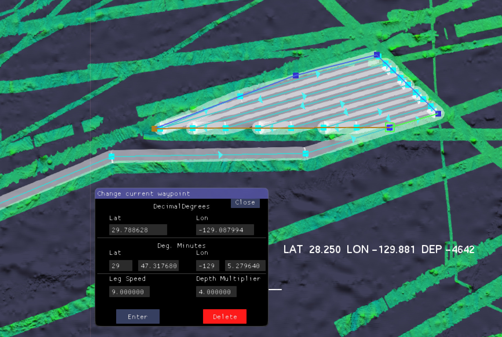
To manually plan a transit, the user enters “Add Waypoints” mode with a pull-down menu selection. In this mode, waypoints may be added by clicking on the map. As waypoints are added, the application computes what the sonar coverage (swath width) would be for a given system specifications and water depth and the estimated coverage is displayed as a transparent overlay. Empirically derived or modelled swath coverage curves as a function of depth can be input into the application, or a simple water depth multiplier entered. Since GapFiller will mostly be used to fill regions where multibeam coverage does not exist, the estimated swath will normally be computed based on satellite-derived predicted bathymetry. Where planned track lines overlap existing mapped areas, the estimated coverage will be based on the directly measured depths (typically using a multibeam echosounder) and the overlap calculation will be more accurate.

Once waypoints have been added, the user can select “Edit Waypoints” mode making it possible to adjust the waypoints by simply clicking and dragging. This also brings up an interface panel whereby a selected waypoint can be deleted or moved to an exact location by entering geographic coordinates. At any point the user can return to “Add Waypoints” mode and add to the end of the planned track, or insert waypoints into an existing segment. A pre-determined list of waypoints file can also be input as a CSV or TXT file.

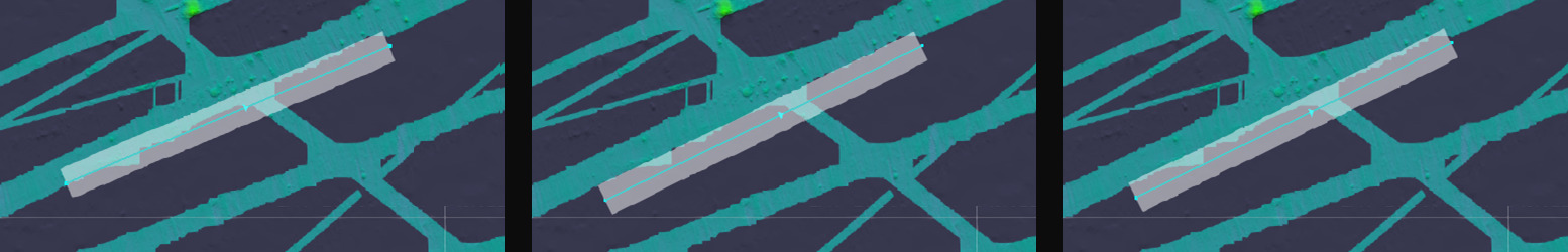
If a segment has been laid alongside a previously mapped line, its overlap can be adjusted by the user hitting the ‘o’ key. This causes the waypoints at either end to be shifted orthogonal to the line so as to achieve a specified amount of overlap using a method described in the algorithms section of this paper (Figs. 1 and 2). This capability will normally be used in “Edit” mode allowing a user to rapidly select and adjust a transit design to edge overlap existing mapping.

Transits can also be planned automatically using a special menu. The user first defines the start and end points which causes a great circle line to appear with distance computed and displayed. Other menu selections result in an automatic transit plan being computed in one of two modes; one generates a set of waypoints designed to maximize the amount of new mapping without regard to existing lines, the other computes a set of waypoints designed to produce lines that slightly overlap existing lines. It is this capability that makes BathyGlobe GapFiller a particularly useful tool for rapidly planning long transects that maximize the coverage of unmapped regions.

Other capabilities of BathyGlobe GapFiller are:

1. Polygon filling – GapFiller allows the user to draw a polygon, which can then be filled automatically with planned track lines. As polygons are filled, the overlap of successive swaths is automatically adjusted based on local depth estimates. Multiple polygons can be linked to form a survey plan (Fig. 1).
2. Survey statistics – GapFiller can compute mapping statistics, based on a transit or survey plan. These include total area mapped, overlap with existing mapping, self-overlap, area of new mapping, time to complete the survey based on an assumed survey speed (which can be adjusted), and an “estimated cost” for the survey based on an input day rate for the vessel (which can also be adjusted). While it is understood that the actual cost of surveying is a complex calculation, we have added this feature to allow the user to get a quick feel for relative costs of different survey options if they have a reasonable idea of the day rate of their platform.

3 Computational methods

BathyGlobe GapFiller incorporates a method for estimating the coverage of planned survey lines as well as an algorithmic method for adjusting planned line segments so that they partially overlap existing segments by a specified percentage. These capabilities can be applied in interactive line planning and are the basis for both automatic transit planning and defining a set of lines to fill a polygonal region.

In the following sections the algorithms for computing swath area estimates, for adjusting overlap, for automatic transit planning and for polygon filling are described in detail.

3.1 Computing swath estimates

Once a track line has been defined a set of discrete sample points are computed by interpolation along the line with a spacing approximating the beam footprint in the along-track direction. These points can be thought of as ship locations for virtual pings. For each point a swath boundary to the port and the starboard side is computed based on the extinction curve for the particular multibeam system that is to be used and on the estimated depth based on the underlying bathymetry. An extinction curve describes how the beam width of a particular MBES decreases with depth (e.g. MAC 2023; Candio et al, 2021; Kongsberg, 2011). The swath limits to either side of the vessel are estimated using a binary search to find the point at which the extinction curve intersects with either previously measured or predicted bathymetry. Figs. 1, 2, 4, 8 and 9 show swath coverage estimated in this way.

3.2 Automatic overlap adjustment

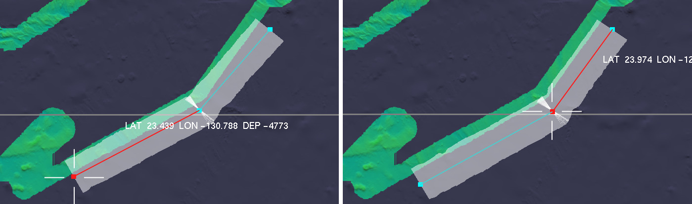
BathyGlobe GapFiller provides automatic adjustment of a planned track line to achieve a specified degree of overlap with existing multibeam mapping data (Fig. 2). Two novel methods for this have been developed and implemented. The first is based on linear regression and the second on a custom overlap detecting filter. Although the first, was demonstrated far less useful than the second, we briefly discuss it here because it is the more obvious solution, and we hope that in describing its shortcomings we may forestall others from following this path. Because of problems with this first regression method, we later developed the filter method which proved to be superior.

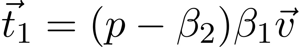
Both methods assume that a transit segment has been defined that partially overlaps a previously mapped line based on the computed swath estimate. The regression-based method computes two regression lines R1 and R2 as illustrated in Fig. 3. R1 approximates the boundary of the planned swath, R2 approximates the edge of the overlap region. The two sets of regression parameters are then used to adjust the waypoints or achieve the desired level of overlap. More detail is provided in Appendix 1.

3.3 Feature detection-based method

Because of the problems with the regression-based method a second algorithm was developed for automatic overlap adjustment using techniques derived from image processing (e.g. Dougherty, 2020). It is based on a custom edge detecting filter and it has proven to be more robust and reliable.

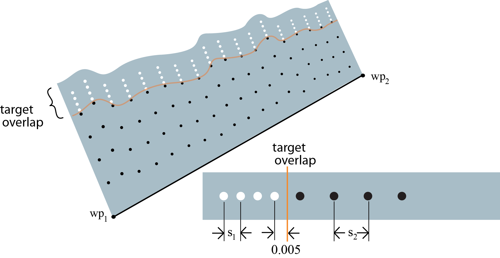
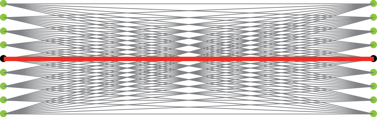
The overlap edge detecting filter incorporates arrays of samples designed to give the strongest response when the filter overlaps an existing multibeam mapped edge by a designated amount. As shown in Fig. 4, the sampling is based on the shape of a proposed swath. Its sampling pattern is asymmetric with sample points more widely spaced on the unmapped side than on the previously mapped side. This asymmetry biases to increase the overlap when the boundary of prior bathymetry is irregular and reduces gaps. When a previously mapped swath is perfectly straight it has no effect on overlap.

If a raster digital map of the seafloor is labelled such that all mapped regions are given a value of +1 and all unmapped regions are given a value of -1, the filter’s response will be maximal when the edge overlaps by the specified amount.

The custom overlap filter is illustrated in Fig. 5. The Overlap function is computed using Eq. (1), where att is a function that returns a value at a sample point from a raster attribute map of the seafloor, c_i represents a point along the planned track, w_i represents the estimated swath width at the sample point, s₁ is the spacing of samples on the overlap side (white in Fig. 4), s₂ is the sample spacing on the non-overlap side (black in Fig. 4). If the raster attribute map of the seabed has a value of +1 where prior multibeam mapping exists and -1 where it does not, the function Overlap returns a value between +1 and -1 being maximal when the designated degree of overlap is attained.

(1)

In practice we have obtained good results using the spacing parameters s₁ and s₂ set to 1 % and 5 % of the swath width respectively. The value of 0.005 (representing half a percent of the swath width) is an arbitrary small amount designed to separate the positively weighed sample points from the negatively weighted sample points.

3.4 Overlap adjustment

The overlap filter is applied using a brute force computational approach. Two sets of test waypoints are calculated using lateral offsets from waypoints wp₁ and wp₂. The product of these two sets is used to generate a set of possible lines illustrated in Fig. 6 and each of these is tested with the overlap filter to find the maximum result. The spacing of the test points is 1 percent of the swath width and values ranging between ± 20 % of the swath width are tested at both ends of the line. This results in 41 × 41 = 1,681 potential lines being evaluated. Greater precision could be achieved by decreasing the spacing, though at increased computational cost.

Whichever test line returns the strongest response replaces the original line.

3.5 Automatic transit planning

The automatic transit planning algorithm generates a series of waypoints defining a transit. It is designed to maximize the number and length of transit segments that partially overlap previously mapped bathymetry by a designated amount. At the same time, it minimizes additional costs in terms of distance travelled. The method is similar to the overlap adjustment algorithm, but with a much coarser sampling to find previously mapped lines to partially overlap. Once the best candidate has been found, the overlap adjustment method is applied. The candidate line is tested with both shorter and longer variants to find the optimal length.

Given transit start and end points entered by the user, the algorithm proceeds with the following steps.

1. Compute a great circle line between the start and end points.
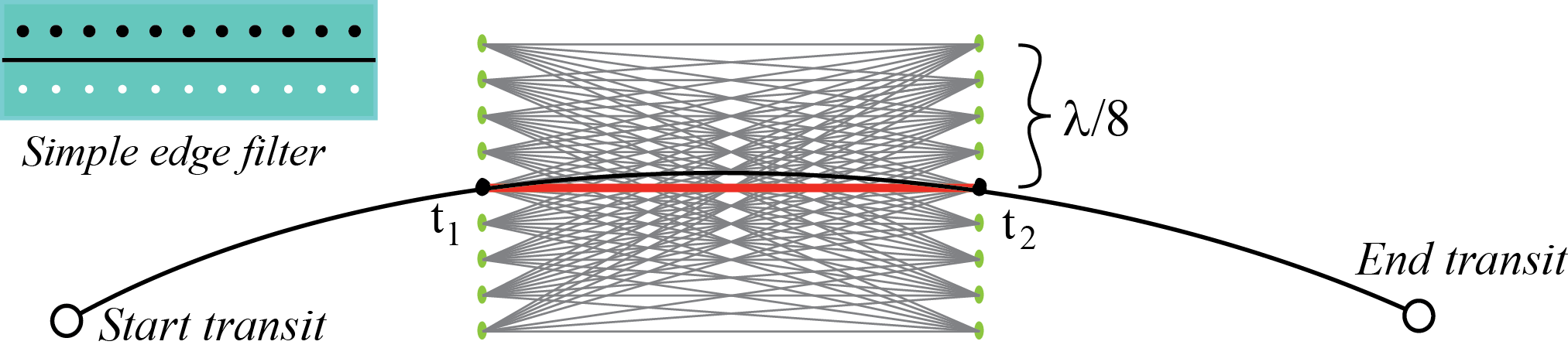
2. On the great circle line compute points t₁ and t₂ at ⅓ and ⅔ of the distance between the start and end points (Fig. 7).
3. Compute a set of test lines in the vicinity of line (t₁ ,t₂) as shown in Fig. 7. The test lines are based on a set of sample points spaced by ¼ of the swath width to the left and right of points t₁ and t₂.
4. For each test line, apply the simple edge filter illustrated in Fig. 7. This has along-track sampling of 8 points per degree. The lateral spacing of sample points to the left and right is ¼ of the swath width. The return value is weighted by two inverted parabolic functions based on the distances from t₁ and t₂ so that lines closest to the great circle are given higher weights.
5. Continue with the test line that returns the largest positive response.
6. Use the overlap adjustment method to refine the line to yield the required overlap percentage.
7. The candidate line is extended or shortened by evaluating candidate test lines in steps of ⅒^th of a (great circle) degree to find the maximal value according to the overlap filter. Once this step is completed the transit segment is set and the algorithm moves on.

To complete the transit, exactly the same process is repeated between the transit start and the beginning of the center segment, and between the end of the center segment and the transit end point. The edge overlapping lines discovered by the method are linked together and line segments are created to the start and end points of the transit. An example transit generated in this way is illustrated in Fig. 8.

The two methods were evaluated by hydrographers skilled in survey planning in a study described in Appendix 2. The results strongly support our choice of the second method, based on feature detection. Fig. 5 shows two examples of both methods where the regression method performs poorly and the feature detection-based method performs well.

3.6 Automatic polygon filling

BathyGlobe GapFiller also enables the user to define a polygonal boundary for full-coverage area surveys. Following this, either of two types of fill can be requested of the software. Both result in sets of lines constructed to fill the polygon with a specified amount of overlap.

Parallel line spacing is the norm for surveying polygonally defined areas (e.g. HYPACK, 2021).The simple fill sets up line spacings where lines are parallel and the spacing is based on the average of the depths at the two end points of the previous line.

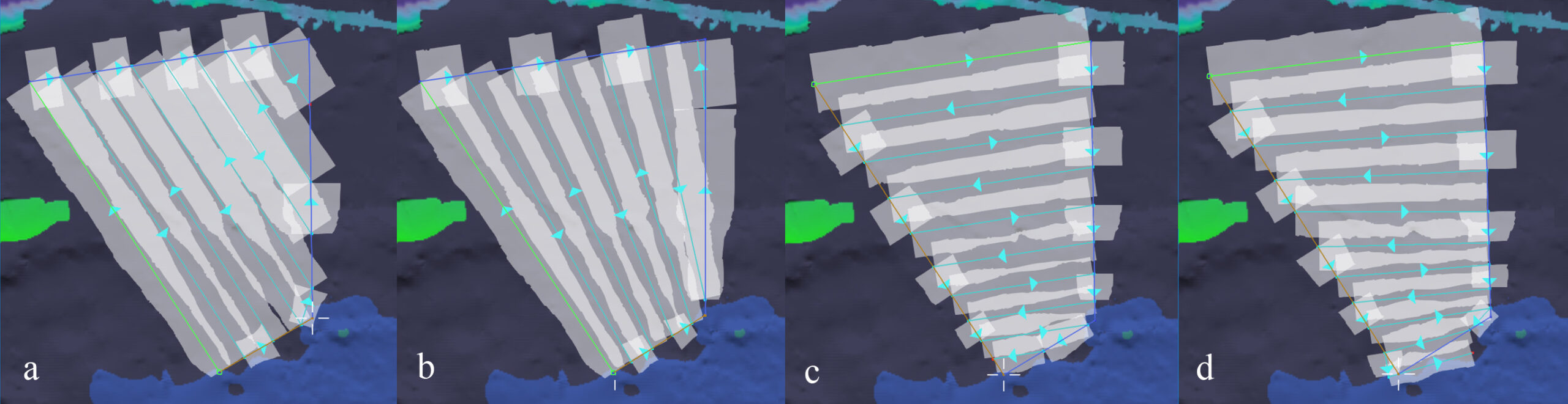
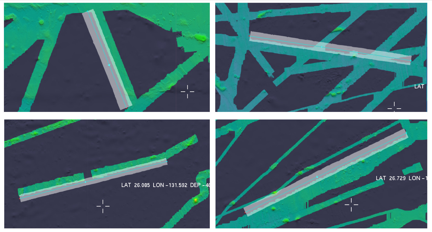
If the ‘extra’ fill option is selected, the overlap adjustment method is applied to each line as it is laid down. This improves coverage where the seafloor in the area varies with depth. Fig. 9 shows two examples of polygon fills with and without the extra adjustment. In Fig. 9a, the lines are parallel and oriented up and down slope. This results in too much overlap at the deep end of the polygon and too little overlap at the shallower end. When overlap adjustment is selected (Fig. 9b) the result is a fan shaped set of lines with much more uniform overlap. Figs. 9c and 9d show the results when the initial line is across-slope. In this case the differences are less marked, although overlap adjustment still results in somewhat more uniform coverage. However, it also results in non-parallel lines. By exploring these options, the user can quickly determine the most efficient orientation to run a survey while maintaining required overlap.

3.7 Coverage calculation

The BathyGlobe GapFiller estimates coverage for a planned survey, generating statistics for new coverage, as well as the amount by which the planned survey will overlap previously mapped areas.

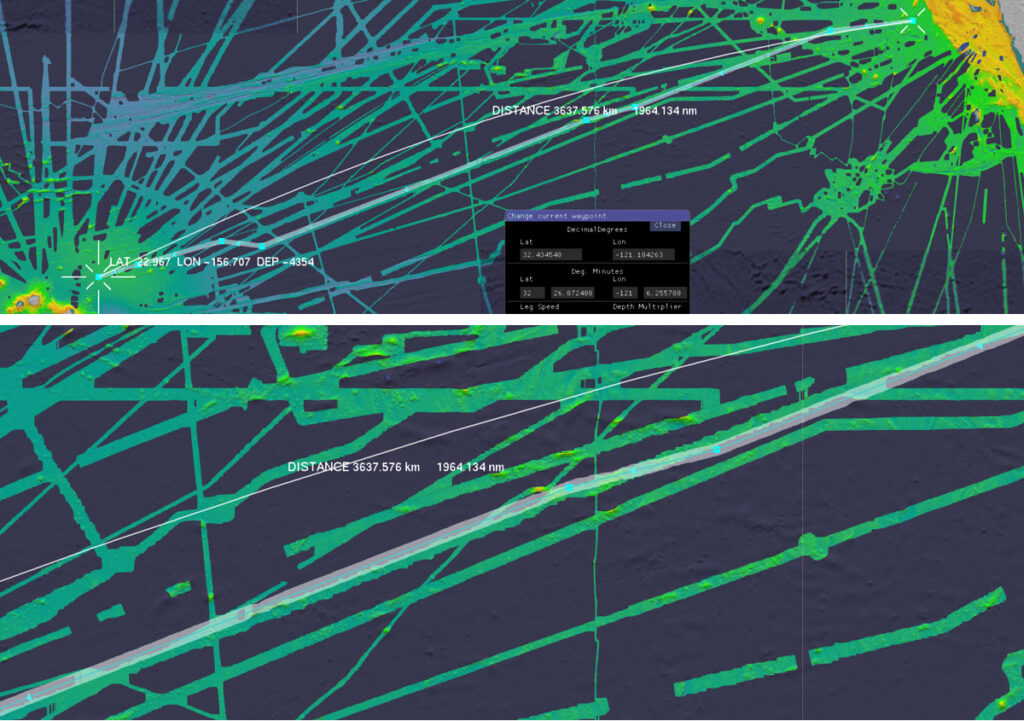
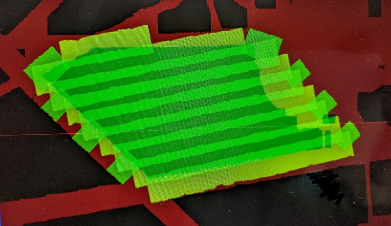
The method used involves setting set up a graphics projection so that each 15 arc sec. GEBCO grid cell is mapped to exactly one pixel of the frame buffer. The planned survey is then drawn in a way that makes use of the color channels of the frame buffer. GEBCO regions that have multibeam data are displayed in the red frame buffer channel and planned multibeam mapping is displayed transparently in the green frame buffer channel. Fig. 10 shows an example. Coverage is estimated by retrieving the contents of the frame buffer and counting pixels classified according to their color content. Pixels that have both red and green indicate overlap of new mapping with prior mapping. Pixels that have only green colors represent new mapping and pixels with a lighter green represent self-overlap. Area mapping statistics are calculated by counting pixels of each type and correcting for latitude (because the area of GEBCO grid cells increases with latitude). Total area mapped is the sum of the areas represented by green pixels. To calculate new mapping, the area represented by pixels having both red and green colors is subtracted. The area of self-overlap is calculated from the light green pixels.

3.8 Survey efficiency calculation

The estimated ship time in days required to complete the transit or survey polygon entered with the predetermined overlap is calculated and displayed whenever the ‘Stats’ menu option is selected. This is calculated based on entered parameters for ship speed and the MBES extinction curve defined in the config file. The user is also allowed to enter a day-rate for the survey platform, if known which allows a quick estimate of survey cost simply based on distance traveled during the survey divided by the ship speed and multiplied by the entered day rate.

Sometimes a survey planner may have the option of contracting with different suppliers who have access to ships with different MBES systems. GapFiller can be used to provide a rough comparison of survey efficiency and costs for different MBES and ship day rates. In order to compare costs for a polygonal area, the area should first be defined and saved. Following this the config file can be set with the parameters (day rate, speed, and extinction file) for each system and the polygon filled for each instance in the usual way.

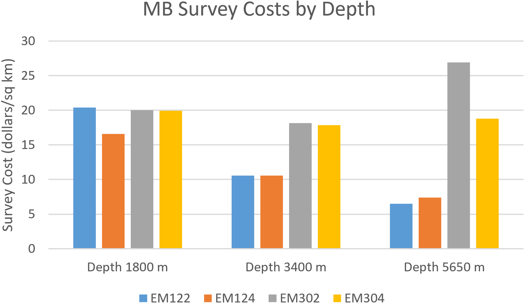
Fig. 11 shows an example of the costs for surveying three different areas with four different MBES systems using a standard ship day rate of $ 45,000, using a 20 % overlap setting and surveying at 9 knots. Each of the areas was approximately 40,000 km2 and their mean depths averaged approximately 1,800 m, 3,400 m and 5,650 m respectively. The survey cost is given in dollars per square meter. The MBES extinction curves came from various sources: The EM124 and EM304 curves are empirical and come from a method developed by the Multibeam Advisory Committee (MAC, 2023). The EM302 curve is based on a hand fit to measurements made on the E/V NAUTILUS (L. Gee, personal comm.). The EM122 curve is a theoretical curve provided in the Product Description document from the manufacturer – Kongsberg Maritime (Kongsberg, 2011). There has been no attempt to standardize these results for such variables as bottom type and water temperature. Consequently, they are given as examples only and should not be used to provide support for an actual cost analysis, but they are quite informative when considering tradeoffs among various MBES systems and the water depths they may be used in.

4 Conclusion

BathyGlobe GapFiller has proven to be useful in rapid interactive multibeam survey planning. It can automatically estimate swath coverage, generate fill patterns for survey polygons, estimate survey times and costs (based on a simple assumption of day-rate), and generate transit paths with edges overlapping previously mapped lines.

One of the most innovative features in GapFiller is an algorithm to provide automatic adjustment of survey lines so that they overlap prior mapping data by a specified amount. This feature is used in both transit planning and polygon filling. Two methods for accomplishing this were implemented, one based on regression, the second based on a custom overlap detecting filter. The filter based method was more successful and is recommended. It derives from a standard technique used in image processing, namely edge detection using a convolution filter, and adapts it to the needs of survey planning. The customized edge detecting filter incorporates the predicted MBES coverage based on estimates of water depth, either from predicted bathymetry based on satellite altimetry (Smith & Sandwell, 1997) or from prior mapping. The sampling pattern within the filter is shaped by this coverage estimate. The algorithm is computationally intensive, relying on a brute force testing of many possible lines. However, because of the speed of modern computers the results are produced in a fraction of a second resulting in fluid interaction experience during path planning.

Nothing reported in this paper is proprietary. Indeed, we support the use of the algorithms and methods presented here and will be happy to offer advice, source code and other assistance to individuals or companies wishing to incorporated them. We have not, however, provided an on-line repository of the source code because it is continuously evolving.

References

Becker, J. J., Sandwell, D. T., Smith, W. H. F., Braud, J., Binder, B., Depner, J. and Ladner, R. (2009). Global bathymetry and elevation data at 30 arc seconds resolution: SRTM30_PLUS, Mar. Geod., 15(32), 355–371.

Bird, J. S. and Mullins, G. K. (2005). Analysis of swath bathymetry sonar accuracy. IEEE Journal of Oceanic Engineering, 30(2), 372–390.

Beaudoin, J. D., Clarke, J. H. and Bartlett, J. E. (2004). Application of surface sound speed measurements in post-processing for multi-sector multibeam echosounders. The International Hydrographic Review, 5(3), 17–32.

Candio, S., Hoy, S., Lobecker, M. and Jerram, K. (2021). NOAA Ship Okeanos Explorer EX-21-01 EM 304 MKII Sea Acceptance Testing Report. https://repository.library.noaa.gov/view/noaa/31024 (accessed 3 Oct. 2023).

Dougherty, E. R. (2020). Digital image processing methods. CRC Press.

Galceran, E. and Carreras, M. (2012). Efficient seabed coverage path planning for ASVs and AUVs. 2012 IEEE/RSJ International Conference on Intelligent Robots and Systems, Vilamoura-Algarve, Portugal, 2012, 88–93. https://doi.org/10.1109/IROS.2012.6385553.

GEBCO (2022). GEBCO Compilation Group Grid. https://doi. org/10.5285/e0f0bb80-ab44-2739-e053-6c86abc0289c HYPACK (2021). HYPACK User Manual. https://www.hypack.com/File%20Library/Resource%20Library/Manuals/2021/ HYPACK-2021-User-Manual.pdf (accessed 18 Aug. 2023).

IBCAO (2023). International Bathymetric Chart of the Arctic Ocean (IBCAO). https://www.gebco.net/data_and_products/gridded_ bathymetry_data/arctic_ocean/ (accessed 3 Oct. 2023).

Jakobsson, M., Mayer, L. A., Bringensparr, C. et al. (2020). The International Bathymetric Chart of the Arctic Ocean Version 4.0. Sci Data, 7, 176. https://doi.org/10.1038/s41597-020-0520-9

Kongsberg (2011). EM122 Multibeam Echo Sounder: Product Description. Report 302440/E. https://epic.awi.de/ide/ eprint/45364/1/Kongsberg_302440ae_em122_product_description.pdf (accessed 22 Sept. 2023).

Kongsberg (2023). Multibeam survey planning. Kongsberg Technical Note. https://www.kongsberg.com/globalassets/maritime/ km-products/product-documents/em-technical-note-multibeam-survey-planning-the-key-to-success.pdf (accessed 18 Aug. 2023).

Li, D., Wang, P. and Du, L. (2018). Path planning technologies for autonomous underwater vehicles – A review. IEEE Access, 7, 9745–9768.

Lucieer, V., Picard, K., Siwabessy, J., Jordan, A., Tran, M. and Monk, J. (2018). Seafloor mapping field manual for multibeam sonar. In R. Przeslawski and S. Foster (Eds.), Field Manuals for Marine Sampling to Monitor Australian Waters (Version 2, pp. 42–64). Report to the National Environmental Science Program, Marine Biodiversity Hub. Geoscience Australia and CSIRO. Canberra, Australia, National Environment Science Programme Marine Biodiversity Hub, 327pp. http:dx.doi. org/10.11636/9781925848755

Manda, D., Thein, M. W. and Armstrong, A. (2015). Depth adaptive hydrographic survey behavior for autonomous surface vessels. OCEANS 2015 MTS/IEEE Washington, Washington, DC, USA, 2015, 1–7. https://doi.org/10.23919/OCEANS.2015.7401831

Mayer, L., Jakobsson, M., Allen, G., Dorschel, B., Falconer, R., Ferrini, V., Lamarche, G., Snaith, H. and Weatherall, P. (2018). The Nippon Foundation – GEBCO seabed 2030 project: The quest to see the world’s oceans completely mapped by 2030. Geosciences, 8(63), 1–18.

MAC (2023). Multibeam Advisory Committee. https://mac.unols. org/system/ (accessed 18 Aug. 2023).

R2Sonic (2023). Multibeam Surveying. https://www.r2sonic.com/wp-content/uploads/2020/03/Multibeam-Surveying.pdf (accessed 18 Aug. 2023).

Smith, W. H. F. and Sandwell, D. T. (1997). Global seafloor topography from satellite altimetry and ship depth soundings. Science, 277, 1957–1962.

Appendix 1: Regression method

The first method we developed to automatically adjust the overlap of planned lines with previously mapped lines was based on linear regression. The method involves first estimating the swath from a planned line as described in the body of the paper. Next a line is fit through the boundary of this swath on the side where it overlaps an existing swath. Following this we compute the amount of overlap of the planned swath as a proportion of the width of the existing swath converted to meters, and a regression line in fit through the overlap boundary. Note: the regressions calculated in meters, with rotated coordinates, the x axis being defined by the original proposed track line, and the y axis orthogonal to it.

In outline, the regression method has the following steps:

1. Compute a swath estimate as described in Section 3.1. Sample along the left and right edges of the swath to determine if there is more overlap with existing multibeam coverage to the left or the right (the method is the same for the feature detection-based method).
2. If there is little overlap or minimal difference between the left and the right overlap no track adjustment occurs.
3. If (left overlap)
   • Compute a linear regression line through the estimated swath boundary on the left hand side (regression R1 in Fig. 3 left).
   • For each ping along the left hand bound ary, compute a set of points where the overlap ends as a proportion of the planned swath width. Compute a linear regression line through the overlap boundary (regression R2 in Fig. 3).
4. Else (right overlap)
   • Compute a linear regression line through the estimated swath boundary on the right hand side.
   • For each ping along the right hand boundary, calculate where the overlap ends. Compute a linear regression line through the overlap boundary.
5. Use the two sets of regression parameters to compute waypoint adjustments to achieve the desired level over overlap as diagrammed in Fig. 3 (right).
6. Re-compute the swath estimate based on the adjusted waypoints.

The waypoint adjustments are determined by the following equations:

R1 (linear fit to boundary of planned swath in meters prior to adjustment)

(2)

R2 (linear fit to prior overlap boundary as a proportion of the swath width)

(3)

Where x corresponds to the distance along the planned track line. If x is scaled between 0 and 1 between the defining waypoints, translations 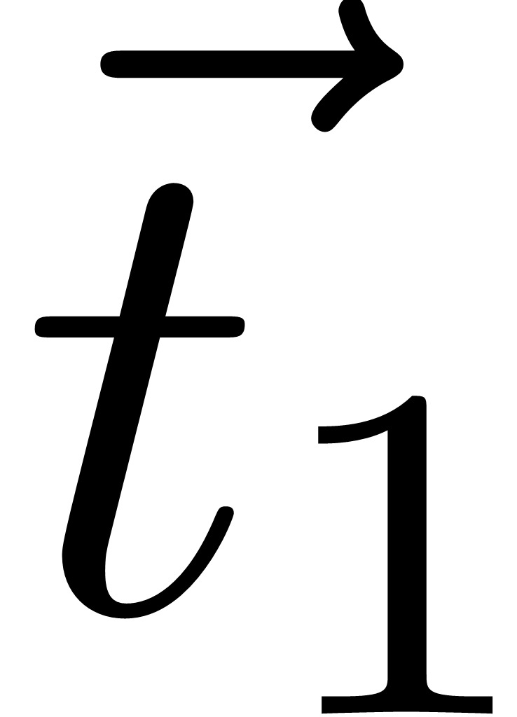and 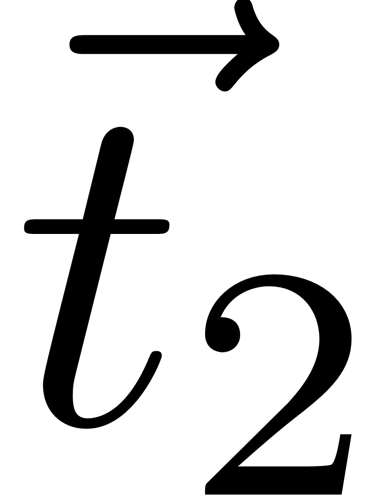at waypoints wp1 and wp2 respectively are given by

(4)

(5)

Where p is the designated overlap as a proportion of swath width and is a unit vector orthogonal to the planned line.

In some cases, this method performed poorly (Appendix 2). We believe that its problems derive from the fact that linear regression is a least squares method and because of this outlying points are over weighted. The poor performance occurs where there are gaps and irregularities in existing multibeam coverage, as well as prior cross tracks. We attempted to remedy some of these issues with piecemeal fixes, such as detecting and excluding gaps. However, this burdened the code with too much complexity and rendered it prone to erratic unpredictable behaviour.

Appendix 2: Evaluation of overlap adjustment methods

In order to evaluate which of the two automatic adjustment methods was more effective we carried out a study in which three NOAA corps officers, skilled in multibeam survey planning, rated the results of automatic overlap adjustments made by the two methods.

Method

30 test lines were created each producing a swath which partially overlapped a previously mapped swath. These lines were chosen to exemplify a variety of different conditions. (1) Simple lines where the existing mapped swath was clean and had no gaps or other lines crossing – this is the base case where both of the methods could be expected to perform well. (3) Lines where prior mapping had crossing lines – this is commonly the case. (2) Lines where existing mapping had gaps. (4) Lines with ragged edges. Each of these is illustrated in Fig. 12.

Each of the test lines was adjusted using both the two methods with a target overlap parameter set at 20 %. Screen shots were captured of the results. The resulting images were placed in pairs on PowerPoint slides with random left right assignment of the two conditions.

For each example, study participants were required to rate the goodness of overlap by the following two criteria. Is the overlap around 20 %? Is the overlap uniform along the length of the swath? Rating was done using a 7 point Likert scale. In addition, participants were required to say whether the left or right example was a better solution or if there was no quality difference in quality.

Results

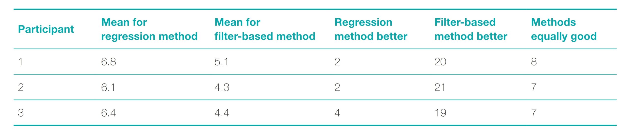
There was only instance where all three of the judges rated the regression method better, whereas there were 18 where all three judges rated the overlap method better. All 30 of the mean ratings for the filter based method were greater than 5 (of 7) and all but three were greater than 6. In comparison only 15 of the mean ratings for the regression method were greater than 5 and only 7 were greater than 6.

Because the ratings data were not close to being normally distributed, non-parametric binomial tests were applied to compare the goodness rating for the two methods using the data in Table 1, columns 3 and 4. For each of the three participants the preferences for the filter method was significantly greater with p < 0.001.

Authors’ biographies

Colin Ware is Professor Emeritus at the University of New Hampshire. He is the former Director of the Data Visualization Research Lab which is part of the Center for Coastal and Ocean Mapping (CCOM) at the University of New Hampshire. Ware holds advanced degrees in both computer science (M.Math, Waterloo) and in the psychology of perception (Ph.D., Toronto). Ware has published two books relating to data visualization and over 150 articles in the field. He has been responsible for the development of numerous software applications used in ocean mapping and oceanography in general.

Larry Mayer is Professor and Director of The Center for Coastal and Ocean Mapping at the University of New Hampshire. His research deals with sonar imaging and remote characterization of the seafloor, advanced applications of 3-D visualization to ocean mapping problems, and applications of mapping to Law of the Sea issues, particularly in the Arctic.

Paul Johnson is the Data Manager at The Center for Coastal and Ocean Mapping at the University of New Hampshire. He has an M.S. in Geology and Geophysics from the University of Hawaii at Manoa where he studied the kinematics of the fastest spreading section of the East Pacific Rise. As data manager at CCOM he has been responsible for innovations in the processing and storage of ocean mapping data. Since 2011 he has co-chaired the Multibeam Advisory Committee, leading a community-based effort whose goal is ensuring that consistent high-quality multibeam data are collected across the U.S. Academic Research Fleet.